9.1 Data Cleansing
We need to be sure that the data we use to create our models is reliable and well structured. And for that we are going to carry out a “tedious” data cleansing process. During this process we are going to handle missing values, outliers, obvious inconsistences and dummy variables.
The first step in the modeling process consists of understanding our goals and the data provided to us. Normally we will have documentation about all the data provided. In case we are the ones who collect those data, we need to create the documentation ourselves. It is essential to understand all the variables that we have to determine their importance for the model. Once we understand out data we import the dataset in R to start working on it.
Titanic Example:

Once we have understood our data we are going to import it into R and study quantitatively how the variables behave before carrying out the cleaning. To do this, first check that the data have been imported correctly into R, ensuring that all rows and columns are identified in our data frame.
data <- read.csv("./Data/titanic3.csv", stringsAsFactors = FALSE, na.strings = "")Secondly, we can obtain the structure of our data frame using the str() function to identify the variable types we have.
str(data)## 'data.frame': 1309 obs. of 14 variables:
## $ pclass : int 1 1 1 1 1 1 1 1 1 1 ...
## $ survived : int 1 1 0 0 0 1 1 0 1 0 ...
## $ name : chr "Allen, Miss. Elisabeth Walton" "Allison, Master. Hudson Trevor" "Allison, Miss. Helen Loraine" "Allison, Mr. Hudson Joshua Creighton" ...
## $ sex : chr "female" "male" "female" "male" ...
## $ age : num 29 0.917 2 30 25 ...
## $ sibsp : int 0 1 1 1 1 0 1 0 2 0 ...
## $ parch : int 0 2 2 2 2 0 0 0 0 0 ...
## $ ticket : chr "24160" "113781" "113781" "113781" ...
## $ fare : num 211 152 152 152 152 ...
## $ cabin : chr "B5" "C22 C26" "C22 C26" "C22 C26" ...
## $ embarked : chr "S" "S" "S" "S" ...
## $ boat : chr "2" "11" NA NA ...
## $ body : int NA NA NA 135 NA NA NA NA NA 22 ...
## $ home.dest: chr "St Louis, MO" "Montreal, PQ / Chesterville, ON" "Montreal, PQ / Chesterville, ON" "Montreal, PQ / Chesterville, ON" ...9.1.1 Handling missing values
When we have missing values in a dataset there are several ways to handle them. Let’s start grouping the solutions in two types:
9.1.1.1 Deletion (drastic approach):
If we find missing values, following this approach we will remove the data, either the whole row or the whole column, depending on whether the missing information corresponds more with the case (we will delete that row) or with the variable (we will delete that column). For the deletion by row we have a basic function of R that will eliminate all the cases in which there is at least one missing value that is na.omit(). But we will never delete data only by columns or by rows, it will depend on the percentage of missing values that we identify in each column. A good criterion is to eliminate all the columns that have more than 80% of missing values. Once we have eliminated those columns we will clean the cases with missing values by rows.
9.1.1.2 Imputation:
Inferring the missing values. This consists of adding or replacing missing values with other values, for example a 0 or the average. There are several methods to impute a missing value and the choice of the best method will depend quite a lot on the context of the information.
Fill in any missing value with 0. In this case we can find for example ages or destination equal to 0, so it does not fit well for all missing values of the dataset.
Impute the value with a string. If we impute by the word “unknown,” this word will appear instead of the missing values, but there are many variables for which we could fill with better information. Therefore, the most commonly used option is to replace the values in different ways for each variable.
We can also use some central tendency measure when filling in missing data, and that is to impute them by the mean or by the median. We can take the values that are not missing from the numeric columns and fill in the missing values with the mean of those values.
9.1.2 Handling missing values (deletion)
To start handling missing values from our dataset let’s check how many we have for each variable. To do this we are going to use the is.na() function, let’s see this function applied to the body variable:
head(is.na(data$body))## [1] TRUE TRUE TRUE FALSE TRUE TRUEThis function will return a Boolean vector with TRUE’s for missing values and FALSE’s for filled values. If we need the complementary vector we could obtain it using the expression !is.na().
head(!is.na(data$body))## [1] FALSE FALSE FALSE TRUE FALSE FALSEWe can use the sum() function to count how many NA’s we have in the variable
sum(is.na(data$body))## [1] 1188But this is only informing us about one variable, and we will need to know the amount of missing values we are working with.
Exercise 9.1 Exercise Develop a function that shows us the missing values for each of the variables of any dataset that we introduce as input.
Once we know the missing values we have to work with, we have to decide what to do with them. Remember that one way to handle them was to eliminate the cases with missing values, and we can do this through the na.omit() function. Let’s see how it works comparing the dataset without missing values and the original one
x = na.omit(data)
c(dim(data), dim(x))
## [1] 1309 14 0 14We see that we have 0 values now in our dataset. This is because all cases have at least one missing value. Let see what happens if we delete the missing values by columns:
y = data.frame(t(na.omit(t(data))))
c(dim(data), dim(y))
## [1] 1309 14 1309 7In this case we don’t lose as much information as we did removing the cases with missing values, but we keep wasting information of variables that can be useful. For this reason, we will always try to balance the deletion of columns and rows.
To do this we are going to create a function that remove all columns with more than 80% of missing values and then remove the remaining cases with missing values.
Exercise 9.2 Exercise Develop a function that remove all columns with more than 80% of missing values and then remove the remaining cases.
9.1.3 Handling missing values (imputation)
That’s great! We already know how to deal with missing values from a case-elimination perspective. This would be one of the solutions, but we have already talked about another possible solution: the imputation of missing values. As mentioned above, there are many ways to impute missing values. Let’s start by replacing all NA’s with 0.
data0 = data
data0[is.na(data0)] = 0
datatable(data0)
This is a good method, but we see that, for example, the variable home.dest(destination) is now equal to 0 in many cases, which is not easy to interpret.
Let’s see another imputation option. Now let’s impute NA’s by the word “Unknown.”
dataString = data
dataString[is.na(dataString)] = "Unknown"
datatable(dataString)
The problem now, as you can expect, is the opposite. We are treating numeric variables as characters when imputing by a word. For this reason, we will always try to impute the missing values of each variable considering its characteristics. Let’s see how to do it with the following exercise:
Exercise 9.3 Exercise:
Impute separately the missing values of the variable body by zeros, the missing values of the variable home.dest by the word “Unknown” and the missing values of the variable age by the mean in the variable age.
Hint: To impute by the mean we need to estimate the mean of the variable, but the mean() function will return an error if we have missing values inside the variable. For that reason we have to include a parameter inside the mean() function called na.rm = TRUE.
Note: There are many other imputation methods much more appropriate, statistically speaking, than the ones we have used, but also much more complex. You will see many of this methods in the future, but in the meantime I recommend this paper from the Loyola University to go deeper.
9.1.4 Outliers
There are multiple methods and a lot of literature about outliers. We will understand outliers as an observation (or set of observations) that are inconsistent with the data set. We will see one technique to detect these outliers, the boxplot.
NOTE: Outliers are NOT errors. We must detect and manage them, but not necessarily remove them, this is a statistical decision and depends on each situation.
For variables in which we can assume normality, the boxplot is a well-recognized technique. All the values above or below the whiskers are considered outliers. The upper whisker is calculated by adding 1.5 times the interquartile range to the third quartile, and the lower by subtracting it from the second quartile.
The Interquantile Range is a measure of statistical dispersion, being equal to the difference between 75th and 25th percentiles, or between upper and lower quartiles, \(IQR = Q3 − Q1\). In other words, the IQR is the first quartile subtracted from the third quartile.
Now we are going to see how the boxplot works. We will use the functions boxplot to print the graph, and boxplot.stats to obtain the exact values of the outliers.
x = c(1:50, 90, 150)
boxplot.stats(x)$out
## [1] 90 150boxplot(x)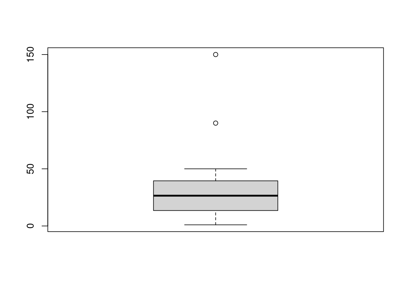
In this case, the values 90 and 150 are considered as outliers as they are above the whisker. We have used a factor of 1.5 to create the whiskers, but we can change this parameter. The more we increase this factor the more we will extend the whiskers, so we include more values inside the range.
boxplot.stats(x, coef = 2)$out## [1] 150The boxplot method fails when data are skewly distributed, as in an exponential distribution. Again, to go deeper in this field I recommend to start reading this paper.
9.1.5 Obvious inconsistencies
An obvious inconsistency occurs when a case contains a value or a combination of values that cannot correspond to reality. For example, a person cannot have a negative age, a man cannot be pregnant, and a child cannot have a driver’s license.
This can be expressed simply through rules or constraints. Checking for obvious inconsistencies can be carried out in R by logical operators. For example, to check that all values of x are not negative we can use the following code.
x = c(-3, 10:20, 30)
xNonNegative = x >= 0
xNonNegative
## [1] FALSE TRUE TRUE TRUE TRUE TRUE TRUE TRUE TRUE TRUE TRUE TRUE
## [13] TRUEHowever, as the number of variables increases, the number of rules increases rapidly, and it may be easier to manage the rules separately from the data. In addition, since rules can be interconnected given certain sets of variables, deciding which variable or variables can create an inconsistency can be complicated.
The editrules package can help us define rules about datasets. In addition, with editrules we will be able to check which rules are fulfilled or not, and it allows us to find the minimum set of values that we have to change to avoid inconsistencies.
We are going to work with a dataset called people.csv to establish our rules. Let’s start by reading the dataset and checking which variables we have
df = read.csv("./Data/people.csv", row.names = "X")
datatable(df)
To check how the library works let’s start by defining some restrictions on the age variable
rules = editset(c("age >= 0", "age <= 150"))
rules
##
## Edit set:
## num1 : 0 <= age
## num2 : age <= 150The editset function analyzes textual rules and stores them in an object we have called rules. Each rule is given a name according to its type (numeric, categorical or mixed). In our example there are only two numerical rules. Now we can verify the data using the function violatedEdits.
violatedEdits(rules, df)## edit
## record num1 num2
## 1 FALSE FALSE
## 2 FALSE FALSE
## 3 FALSE FALSE
## 4 FALSE TRUE
## 5 FALSE FALSEWe can see how the second rule is broken in case 4 of our dataset as it has an age greater than 150 years. This function will return a logical array indicating the possible inconsistencies in the data according to our rules.
As we have said before, the number of rules that we will apply will increase enormously depending on the number of variables in our dataset. However, editrules will make our work easier, being able to write even the list of rules in a text file and introducing it later in R with the editfile function. Here we have an example:
rules = editfile("./Data/rules.txt")
rules
##
## Data model:
## dat6 : agegroup %in% c('adult', 'child', 'elderly')
## dat7 : status %in% c('married', 'single', 'widowed')
##
## Edit set:
## num1 : 0 <= age
## num2 : 0 < height
## num3 : age <= 150
## num4 : yearsmarried < age
## cat5 : if( agegroup == 'child' ) status != 'married'
## mix6 : if( age < yearsmarried + 17 ) !( status %in% c('married', 'widowed') )
## mix7 : if( age < 18 ) !( agegroup %in% c('adult', 'elderly') )
## mix8 : if( 18 <= age & age < 65 ) !( agegroup %in% c('child', 'elderly') )
## mix9 : if( 65 <= age ) !( agegroup %in% c('adult', 'child') )In this file we can see that there are numerical, categorical and mixed, and also univariate and multivariate rules.
In addition, as the number of rules can increase a lot, this library offers us another two functions to summarize the violation of the rules: summary and plot
violatedRules = violatedEdits(rules, df)
summary(violatedRules)
## Edit violations, 5 observations, 0 completely missing (0%):
##
## editname freq rel
## cat5 2 40%
## mix6 2 40%
## num2 1 20%
## num3 1 20%
## num4 1 20%
## mix8 1 20%
##
## Edit violations per record:
##
## errors freq rel
## 0 1 20%
## 1 1 20%
## 2 2 40%
## 3 1 20%plot(violatedRules)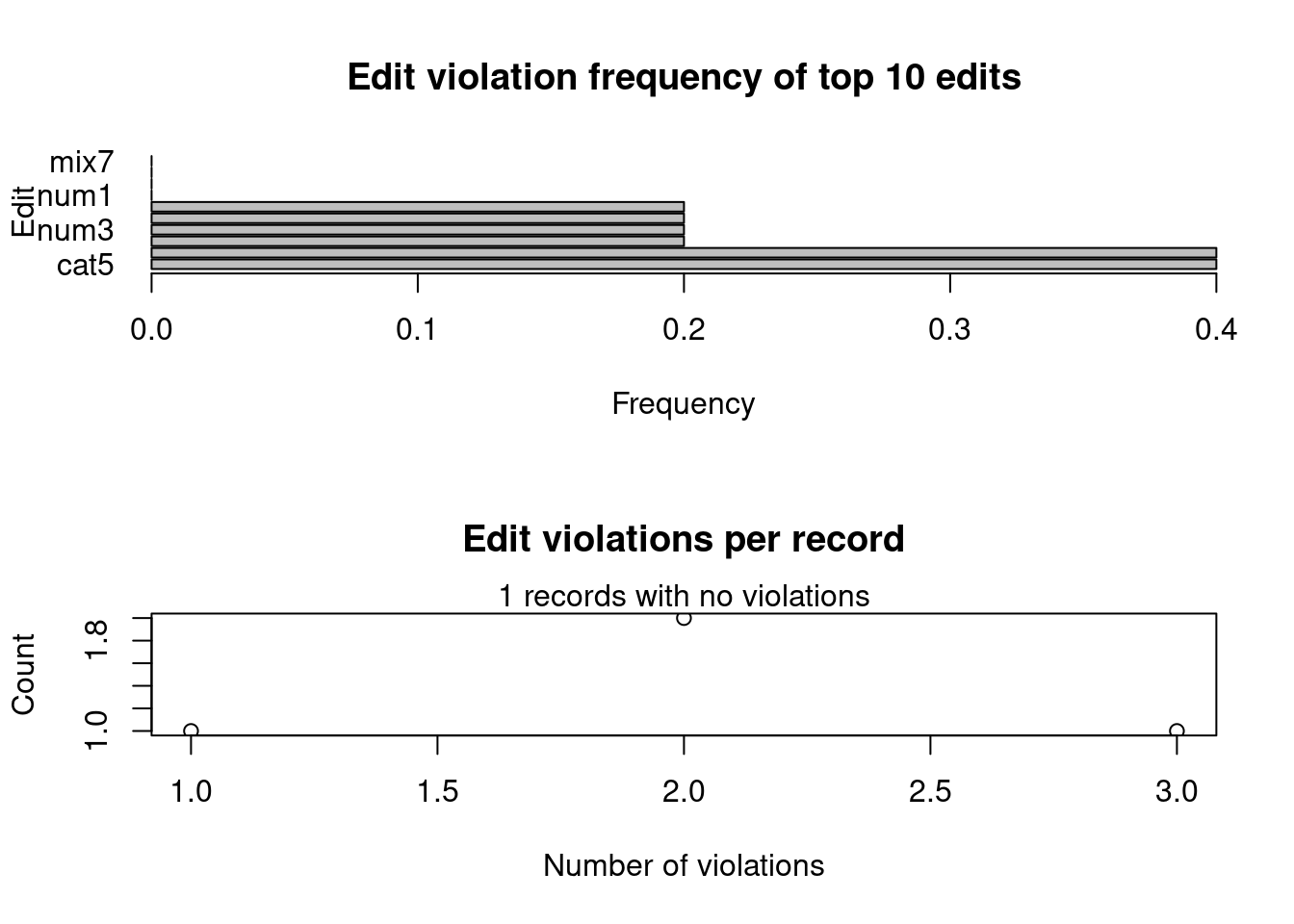
9.1.6 Dummy variables
What does dummifying a variable means? It is a process that consists of creating separate variables for each category when we have a categorical variable. Although categorical variables already contain a lot of information, it is sometimes useful to convert that category into separate columns.
Example with the variable “sex”: this variable defines a category, a classification of each of the rows between men and women. Instead of using this categorical variable we will create two dummy variables, a male column (0,1) and a female one (0,1). What we do is eliminate the categorical variables and create new variables for each category of the variable.
However, we don’t normally need to write all this code to create the dummy variables since R already takes into account the factors as if they were dummy variables in most of R modeling functions. But in case there is a library that does not interpret the factors as dummy variables, we can use this code to dummify the variables.
dummy_sex <- model.matrix( ~ sex - 1, data = data)
datatable(dummy_sex)