2.5 R as a Calculator
The screen prompt > is an invitation to put R to work. You can use the Rstudio command line as a calculator, like this:
log(42/7.3)## [1] 1.749795Each line can have at most 8192 characters, but if you want to see a lengthy instruction or a complicated expression on the screen, you can continue it on one or more further lines simply by ending the line at a place where the line is obviously incomplete (e.g. with a trailing comma, operator, or with more left parentheses than right parentheses, implying that more right parentheses will follow).
When continuation is expected, the prompt changes from > to +:
5+6+3+6+4+2+4+8+
3+2+7
## [1] 50Note that the + continuation prompt does not carry out arithmetic plus. If you have made a mistake, and you want to get rid of the + prompt and return to the > prompt, then press the Esc key and use the Up arrow to edit the last (incomplete) line.
Two or more expressions can be placed on a single line so long as they are separated by semi-colons:
2+3; 5*7; 3-7## [1] 5## [1] 35## [1] -4For very big numbers or very small numbers R uses the following scheme (called exponents):
1.2e3: means 1200 because the e3 means ‘move the decimal point 3 places to the right’1.2e-2: means 0.012 because the e-2 means ‘move the decimal point 2 places to the left’3.9+4.5i: is a complex number with real (3.9) and imaginary (4.5) parts, and i is the square root of –1.
2.5.1 Complex numbers in R
Complex numbers consist of a real part and an imaginary part, which is identified by lower-case i like this:
z = 3.5-8iThe elementary trigonometric, logarithmic, exponential, square root and hyperbolic functions are all implemented for complex values. The following are the special R functions that you can use with com- plex numbers:
- Determine the real part:
Re(z)## [1] 3.5- Determine the imaginary part:
Im(z)## [1] -8- Calculate the modulus (if x is the real part and y is the imaginary part, then the modulus is \(\sqrt(x^2 + y^2)\)):
Mod(z)## [1] 8.732125- Calculate the argument (
Arg(x+ yi)= atan(y/x)):
Arg(z)## [1] -1.158386- Work out the complex conjugate (change the sign of the imaginary part):
Conj(z)## [1] 3.5+8i- Check if the object is a complex number:
is.complex(z)## [1] TRUE- Coerce a number into a complex number:
as.complex(3.8)## [1] 3.8+0i2.5.2 Rounding
Various sorts of rounding (rounding up, rounding down, rounding to the nearest integer) can be done easily. Take the number 5.7 as an example. The ‘greatest integer less than’ function is floor:
floor(5.7)## [1] 5The ‘next integer’ function is ceiling:
ceiling(5.7)## [1] 6You can round to the nearest integer by adding 0.5 to the number, then using floor. There is a built-in function for this, but we can easily write one of our own to introduce the notion of function writing. Call it rounded, then define it as a function like this:
rounded = function(x){floor(x+0.5)}Now we can use the new function:
rounded(5.7)## [1] 6rounded(5.4)## [1] 5There is an R function called round that you can use by specifying 0 decimal places in the second argument:
round(5.7,0)## [1] 6round(5.4,0)## [1] 5round(-5.7,0)## [1] -62.5.3 Arithmetics
The screen prompt in R is a fully functional calculator. You can add and subtract using the obvious + and - symbols, while division is achieved with a forward slash / and multiplication is done by using an asterisk * like this:
7 + 3 - 5 * 2## [1] 0Notice from this example that multiplication (5 × 2) is done before the additions and subtractions.
Powers (like squared or cube root) use the caret symbol ˆ and are done before multiplication or division, as you can see from this example:
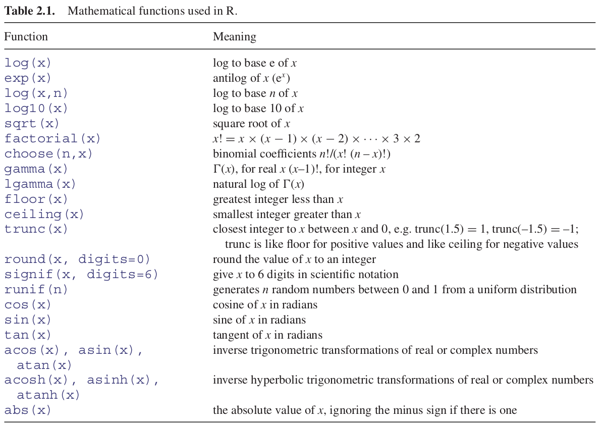
3^2 / 2## [1] 4.5All the mathematical functions you could ever want are here (see Table 2.1).
The log function gives logs to the base e (e = 2.718 282), for which the antilog function is exp:
log(10)## [1] 2.302585exp(1)## [1] 2.718282Logs to other bases are possible by providing the log function with a second argument which is the base of the logs you want to take. Suppose you want log to base 3 of 9:
log(9,3)## [1] 2The trigonometric functions in R measure angles in radians. A circle is \(2\pi\) radians, and this is \(360^\circ\) , so a right angle (\(90^\circ\)) is \(\pi / 2\) radians. R knows the value of \(\pi\) as pi:
pi## [1] 3.141593sin(pi/2)## [1] 1cos(pi/2)## [1] 6.123234e-17Notice that the cosine of a right angle does not come out as exactly zero, even though the sine came out as exactly 1. The e-017 means ‘times \(10^{–17}\).’ While this is a very small number, it is clearly not exactly zero.
2.5.4 Modulo and integer quotients
Integer quotients and remainders are obtained using the notation %/% (percent, divide, percent) and %% (percent, percent) respectively. Suppose we want to know the integer part of a division: say, how many 13s are there in 119:
119 %/% 13## [1] 9Now suppose we wanted to know the remainder (what is left over when 119 is divided by 13): in maths this is known as modulo:
119 %% 13## [1] 2Modulo is very useful for testing whether numbers are odd or even: odd numbers have modulo 2 value 1 and even numbers have modulo 2 value 0:
9 %% 2## [1] 18 %% 2## [1] 0Likewise, you use modulo to test if one number is an exact multiple of some other number. For instance, to find out whether 15 421 is a multiple of 7 (which it is), then ask:
15421 %% 7## [1] 02.5.5 Operators
R uses the following operator tokens:
+ - * / %/% %% ˆ: arithmetic (plus, minus, times, divide, integer quotient, modulo, power)>= < <= == !=: relational (greater than, greater than or equals, less than, less than or equals, equals, not equals)! & |: logical (not, and, or)~: model formulae (‘is modelled as a function of’)= ->: assignment (gets)$: list indexing (the ‘element name’ operator):: create a sequence
Several of these operators have different meaning inside model formulae. Thus * indicates the main effects plus interaction (rather than multiplication), : indicates the interaction between two variables (rather than generate a sequence) and ˆ means all interactions up to the indicated power (rather than raise to the power). You will learn more about these ideas in further sessions.