3.3 Random Variables

Statistics is concerned with data. The concept of a random variable provides the link between sample spaces and events to data.

Definition: A random variable is a mapping \[ X: \Omega \rightarrow \mathbb{R} \]

that assigns a real number \(X(\omega)\) to each outcome \(\omega\). We will basically only work directly with random variables and although the sample space will be barely mentioned, you should keep in mind that it is there!

Example: Flip a coin ten times. Let \(X\) be the random variable counting the number of heads. For example, if \(\omega= HHTHHTHHTT\), then \(X(\omega)=6\).

Example: Let \(\Omega=\{(x,y): x^2+y^2 \leq 1\}\). Consider drawing a point at random from \(\Omega\) (we will make this idea more precise later). A typical outcome is of the form \(\omega=(x,y)\). Some examples of random variables are \(X(\omega)=x\), \(Y(\omega)=y\), \(Z(\omega)=x+y\).

Given a random variable \(X\) and a subset \(A\) of the real line, let

\[\begin{align} \mathbb{P}(X\in A) &= \mathbb{P}(\{\omega\in\Omega: X(\omega)\in A\})\\ \mathbb{P}(X = x) &= \mathbb{P}(\{\omega\in\Omega: X(\omega)=x\}) \end{align}\]

Notice that \(X\) denotes the random variable and \(x\) denotes a particular value of \(X\)

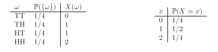
Example: Flip a coin twice and let \(X\) be the number of heads. Then, \(\mathbb{P}(X=0)=\mathbb{P}(\{TT\})=1/4\), \(\mathbb{P}(X=1)=\mathbb{P}(\{TH,HT\})=1/2\) and \(\mathbb{P}(X=2)=\mathbb{P}(\{HH\})=1/4\). The random variable and its distribution can be summarized as follows:

3.3.1 Distribution Functions

Definition Given a random variable \(X\), the cumulative distribution function or CDF is the function \(F_X:\mathbb{R}\rightarrow [0,1]\) defined by

\[ F_X(x)=\mathbb{P}(X\leq x) \]

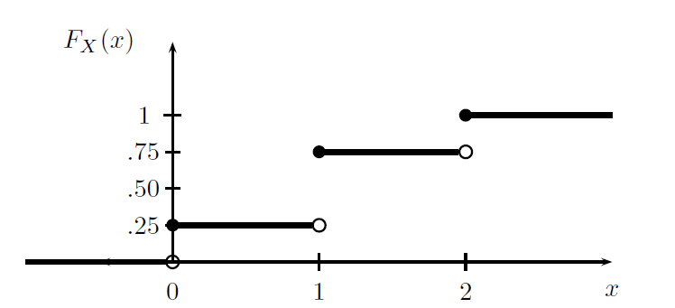
Example: Flip a fair coin twice and let \(X\) be the number of heads. Then \(\mathbb{P}(X=0)=\mathbb{P}(X=2)=1/4\) and \(\mathbb{P}(X=1)=1/2\). The distribution function is

\[ F_X(x)=\left\{ \begin{array}{ll} 0, & x<0\\ 1/4, & 0\leq x <1\\ 3/4, & 1\leq x <2 \\ 1, & x\geq 2 \end{array} \right. \]

The following result shows that the CDF completely determines the distribution of a random variable

Theorem Let \(X\) have CDF \(F_X\) and let \(Y\) have CDF \(F_Y\). If \(F_X(x)=F_Y(x)\) for all \(x\), then \(\mathbb{P}(X\in A)=\mathbb{P}(Y\in A)\) for all \(A\).

Some properties of the CDF are:

• \(F_X\) is non-decreasing: \(x_1<x_2\) implies that \(F_X(x_1)\leq F_X(x_2)\)
• \(F_X\) is normalized: \(\lim_{x\rightarrow -\infty}F_X(x)=0\) and \(\lim_{x\rightarrow +\infty}F_X(x)=1\)
• \(F_X\) is right-continuous
• It is defined for all \(x\in\mathbb{R}\).

3.3.2 Random variable types

There are two fundamental types of random variables, discrete and continuous. The following is a rough definition.

Discrete and Continuous Random Variables

• A random variable is discreet if it can only take a number of values with positive probability.
• Random continuous variables take values in intervals.

Example 3.1 Example

These are discreet random variables:

• number of damaged items in a shipment
• Number of customers arriving at a bank in an hour.
• Number of errors detected in a company’s accounts.
• Number of health insurance policy claims.

These are continuous random variables:

• Annual income of a family.
• Amount of oil imported by a country.
• Variation in the price of a telecommunication company’s shares.
• Percentage of impurities in a batch of chemicals.

3.3.3 Discrete Random Variables

We will now describe the behavior of r.v. To do this we will use different functions that will give us some probabilities of the random variable. In the discrete case these functions are the probability function and the cumulative distribution function. In the discrete case the probability function is the one that gives us the probabilities of the elementary events of r.v.

Definition: \(X\) is discrete if it takes countably many values \(\{x_1,x_2,\dots\}\). We define the probability function or probability mass function for \(X\) by \(f_X(x)=\mathbb{P}(X=x)\).

Thus \(f_X(x)\geq 0\) for all \(x\) and \(\sum_i f_X(x_i)=1\). The CDF of \(X\) is related to \(f_X\) by \[ F_X(x)=\mathbb{P}(X\leq x)=\sum_{x_i\leq x}f_X(x_i) \]

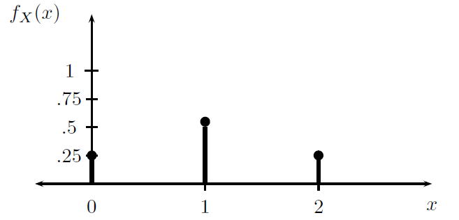
Example: The probability mass function for the example of the toss of two coins is \[ f_X(x)=\left\{ \begin{array}{ll} 1/4, & x=0\\ 1/2, & x=1\\ 1/4, & x=2 \\ 0, & otherwise \end{array} \right. \]

Consider the throw of two dice and define the random variable \(X\) as the absolute difference of the dice results. \(X\) can thus take values \({0,1,2,3,4,5}\). By counting appropriately the possible cases the PMF can be derived as

\[ f_X(x)=\left\{ \begin{array}{ll} 6/36 & x=0 \\ 10/36 & x=1 \\ 8/36 & x=2\\ 6/36 & x=3 \\ 4/36 & x=4\\ 2/36 & x=5 \end{array} \right. \]

3.3.4 Continuous Random Variables

Definition A random variable \(X\) is continuous if there exists a function \(f_X\) such that \(f_X(x)\geq 0\) for all \(x\), \(\int_{-\infty}^{\infty}f_X(x)dx=1\) and for every \(a\leq b\) \[ \mathbb{P}(a<X<b)=\int_a^bf_x(x)dx \] The function \(f_X\) is called the probability density function (PDF). We have that \[ F_X(x)=\int_{-\infty}^xf_x(t)dt \] and \(f_X(x)=F_X^{'}(x)\) at all points \(x\) at which \(F_X\) is differentiable.

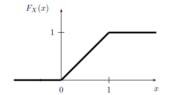
Example: Suppose that \(X\) has PDF \[ f_X(x)=\left\{ \begin{array}{ll} 1, & for \; 0\leq x\leq 1\\ 0, & otherwise \end{array} \right. \]

Clearly, \(f_X(x)\geq 0\) and \(\int_{-\infty}^{\infty}f_X(x)dx=1\). The CDF is given by \[ F_X(x)=\left\{ \begin{array}{ll} 0, & x<0\\ x, & 0\leq x \leq 1\\ 1, & x>1 \end{array} \right. \]

Continuous random variables can lead to confusion. First, note that if \(X\) is continuous then \(\mathbb{P}(X=x)=0\) for every \(x\). Do not try to think of \(f_X(x)\) as \(\mathbb{P}(X=x)\). This only holds for discrete random variables. We get probabilities from a PDF by integrating.

• \(\mathbb{P}(X=x)=0\)
• \(\mathbb{P}(x< X \leq y)= F_X(y)-F_X(x)\)
• \(\mathbb{P}(X>x)=1-F_X(x)\)
• If \(X\) is continuous then \[ F_X(b)-F_X(a)= \mathbb{P}(a<X<b)=\mathbb{P}(a\leq X<b)=\mathbb{P}(a<X\leq b)=\mathbb{P}(a\leq X \leq b) \]

Let’s make a simple example to understand that \(\mathbb{P}(X=x)=0\)

Suppose we have a uniform continuous random variable \(X\) with a PDF:

\[ f_{X}(x)=\begin{cases} \frac{1}{5},\ for\ 0 \leq x \leq 5\\ 0,\ otherwise \end{cases} \]

The plot of the PDF will be:

X = density(runif(9999999, 0, 5))
plot(X, col = "blue", main = "X PDF",xlab = "", xlim = c(-2,7))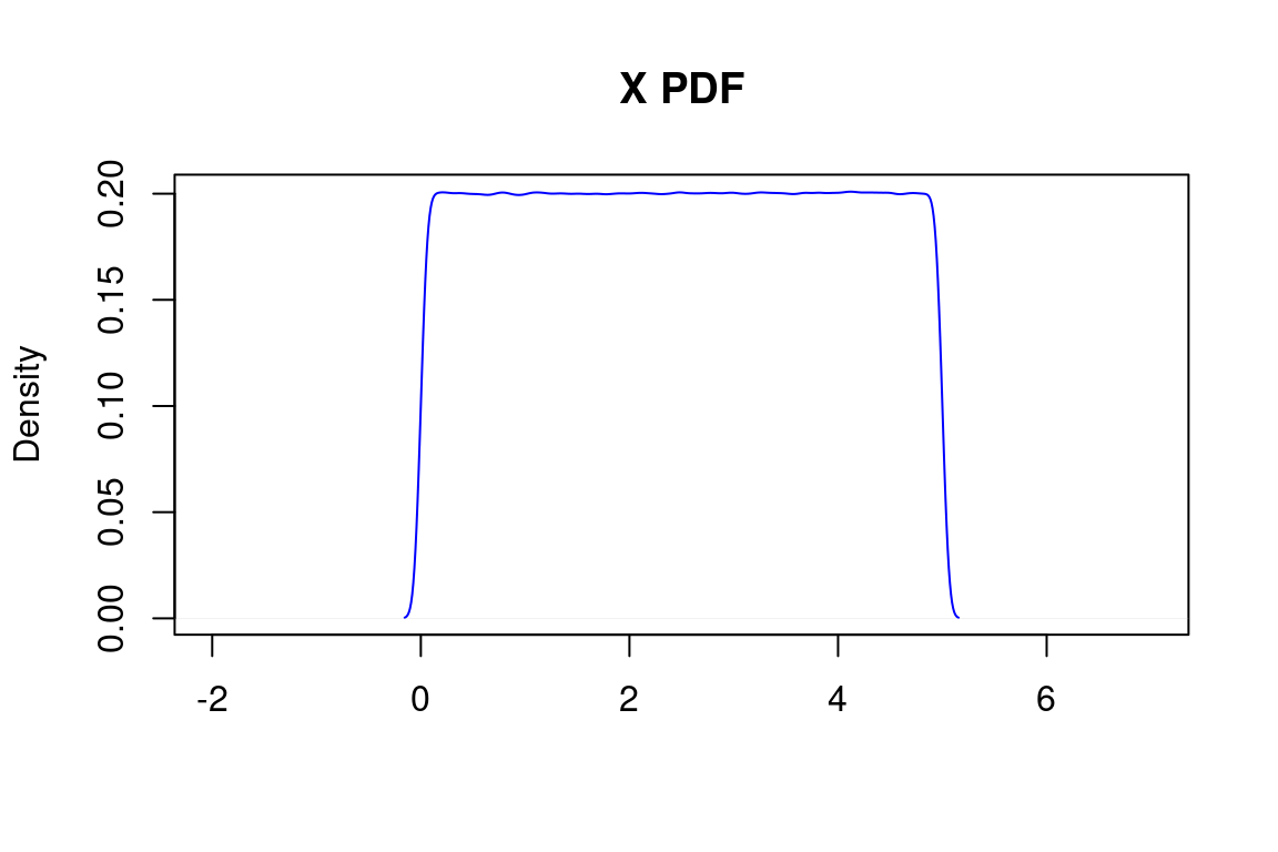

And the CDF is given by: \[ F_{X}(x)=\begin{cases} 0,\ x < 0 \\ \frac{x}{5},\ 0 \leq x \leq 5 \\ 1, x > 5 \end{cases} \]

Since we are working with a uniform distribution, we can assume that the area under the curve is equal to base per height. We already know that the area equals 1, and the base equals 5. This way we can calculate that:

\[\begin{align} AUC = base*height, \\ 1 = 5*height, \\ height = 1/5 = 0.2 \end{align}\]

With this information it will be very easy for us to calculate more specific probabilities. For example, let’s calculate \(\mathbb{P}(1 \leq x \leq 2)\):

\[ \mathbb{P}(1 \leq x \leq 2) = 1*1/5 = 0.2 \]

plot(X, col = "blue", main = "X PDF",xlab = "",xlim=c(1,2))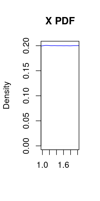

Well, now let’s look at more extreme scenarios. Let’s calculate the following probabilities:

• \(\mathbb{P}(4 \leq x \leq 4.333) = 1/3 * 1/5 = 0.0666\)
• \(\mathbb{P}(2.9 \leq x \leq 3.1) = 1/5 * 1/5 = 0.04\)
• \(\mathbb{P}(2.99 \leq x \leq 3.01) = 1/50 * 1/5 = 0.004\)
• \(\mathbb{P}(2.999 \leq x \leq 3.001) = 1/500 * 1/5 = 0.0004\)
• \(\mathbb{P}(x=3) = 1/\infty * 1/5 = 0\)

3.3.5 Expectation of a Random Variable

The expected value or expectation or mean of \(X\) is defined to be \[ \mathbb{E}(X)=\sum_x xf_X(x) \] if \(X\) is discrete and \[ \int xf_X(x)dx \] if \(X\) is continuous.

The expectation is a one-number summary of the distribution characterizing the average behavior of the random variable.

Example: Flip a fair coin two times. Let \(X\) be the number of heads. Then \(\mathbb{E}(X)=\sum_{x}xf_X(x)= 0\times f_X(0)+1\times f_X(1) + 2\times f_X(2)=0\times 1/4 + 1 \times 1/2 +2 \times 1/4 = 1\).

• For any two random variables \(X\) and \(Y\), \(\mathbb{E}(X+Y)=\mathbb{E}(X)+\mathbb{E}(Y)\).
• For any random variable \(X\) and constant \(a\), \(\mathbb{E}(aX)=a\mathbb{E}(X)\).
• For any constant \(b\), \(\mathbb{E}(b)=b\).
• So more generally \(\mathbb{E}(aX+bY+c)=a\mathbb{E}(X)+b\mathbb{E}(Y)+c\).
• If \(X\) and \(Y\) are independent \(\mathbb{E}(XY)=\mathbb{E}(X)\mathbb{E}(Y)\).

3.3.6 Variance of Random Variables

The variance of a random variable \(X\), denoted by \(\mathbb{V}(X)\), measures the spread of a distribution and is defined by \[ \mathbb{V}(X)=\mathbb{E}((X-\mathbb{E}(X))^2). \] If \(X\) is discrete \[ \mathbb{V}(X)=\sum_x(x-\mathbb{E}(X))²f_X(x) \] and if \(X\) is continuous \[ \mathbb{V}(X)=\int(x-\mathbb{E}(X))f_X(x)dx \] The standard deviation is \(sd(X)=\sqrt{\mathbb{V}(X)}\).

• \(\mathbb{V}(X)=\mathbb{E}(X^2)-\mathbb{E}(X)^2\)
• If \(a\) and \(b\) are constants then \(\mathbb{V}(aX+b)=a^2\mathbb{V}(X)\)
• If \(X\) and \(Y\) are independent \(\mathbb{V}(X+Y)=\mathbb{V}(X)+\mathbb{V}(Y)\).

3.3.7 Sample Mean and Sample Variance

If \(X_1,\dots,X_n\) are random variables then we define the sample mean to be \[ \bar{X}_n=\frac{1}{n}\sum_{i=1}^n X_i \] and the sample variance to be \[ S_n^2=\frac{1}{n-1}\sum_{i=1}^n(X_i-\bar{X}_n)^2 \]

Theorem Let \(X_1,\dots, X_n\) be independent and let \(\mu=\mathbb{E}(X_i)\) and \(\sigma^2=\mathbb{V}(X_i)\). Then \[ \mathbb{E}(\bar{X}_n)=\mu, \qquad \mathbb{V}(\bar{X}_n)=\frac{\sigma^2}{n} \qquad \mathbb{E}(S_n^2)=\sigma^2 \]

3.3.8 Covariance between Random Variables

If \(X\) and \(Y\) are random variables then the covariance and the correlation between \(X\) and \(Y\) measure the strength of their linear relationship.

The covaraince between \(X\) and \(Y\) is defined by \[ Cov(X,Y)=\mathbb{E}\left((X-\mathbb{E}(X))(Y-\mathbb{E}(Y))\right) \] and the correlation by \[ \rho(X,Y)=\frac{Cov(X,Y)}{sd(X)sd(Y)} \]

• The covariance satisfies \[ Cov(X,Y)=\mathbb{E}(XY)-\mathbb{E}(X)\mathbb{E}(Y) \]
• The correlation satisfies \[ -1\leq \rho(X,Y)\leq 1 \]
• If \(X\) and \(Y\) are independent then \(Cov(X,Y)=\rho(X,Y)=0\), but the converse is in general not true.
• If \(Y=aX+b\), then \(\rho(X,Y)=1\) if \(a>0\) and \(\rho(X,Y)=-1\) if \(a<0\).
• It holds that \[ \mathbb{V}(X+Y)=\mathbb{V}(X)+\mathbb{V}(Y)+2Cov(X,Y) \] \[ \mathbb{V}(X-Y)=\mathbb{V}(X)+\mathbb{V}(Y)-2Cov(X,Y) \]