4.6 Testing Generic Simulation Sequences

In previous sections we spent a lot of effort in assesing if a sequence of numbers could have been a random sequence of independent numbers from a Uniform distribution between zero and one.

Now we will look at the same question, but considering generic distributions we might be interested in. Recall that we had to check two aspects:

1. if the random sequence had the same distribution as the theoretical one (in previous sections Uniform between zero and one);

2. if the sequence was of independent numbers

We will see that the tools to perform these steps are basically the same.

4.6.1 Testing Distribution Fit

There are various ways to check if the random sequence of observations has the same distribution as the theoretical one.

4.6.1.1 Histogram

First, we could construct an histogram of the data sequence and compare it to the theoretical distribution. Suppose we have a sequence of numbers x1 that we want to assess if it simulated from a Standard Normal distribution.

x1 <- data.frame(x1 =rnorm(500))

ggplot(x1, aes(x1)) +
   geom_line(aes(y = ..density.., colour = 'Empirical'), stat = 'density') +
   stat_function(fun = dnorm, aes(colour = 'Normal')) +      
   geom_histogram(aes(y = ..density..), alpha = 0.4) +      
   scale_colour_manual(name = 'Density', values = c('red', 'blue')) +
   theme_bw()

## `stat_bin()` using `bins = 30`. Pick better value with `binwidth`.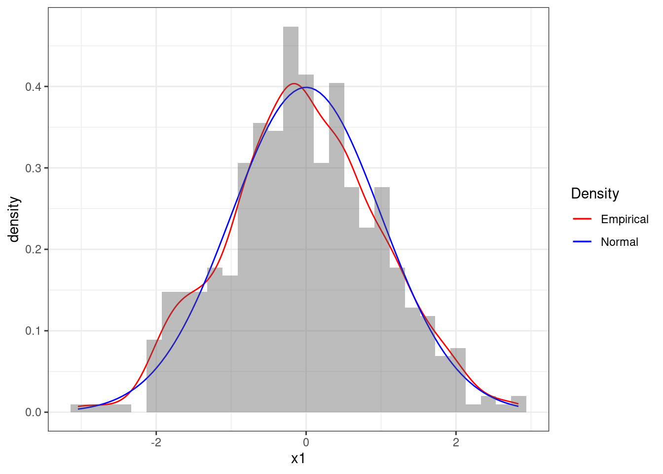

Figure 4.9: Histogram of the sequence x1 together with theoretical pdf of the standard Normal

Figure 4.9 reports the histogram of the sequence x1 together with a smooth estimate of the histogram, often called density plot, in the red line. The blue line denotes the theoretical pdf of the standard Normal distribution. We can see that the sequence seems to follow quite closely a Normal distribution and therefore we could be convinced that the numbers are indeed Normal.

Let’s consider a different sequence x2. Figure 4.10 clearly shows that there is a poor fit between the sequence and the standard Normal distribution. So we would in general not believe that these observations came from a Standard Normal.

x2 <- data.frame(x2 =rnorm(500,0.5,0.6))

ggplot(x2, aes(x2)) +
   geom_line(aes(y = ..density.., colour = 'Empirical'), stat = 'density') +
   stat_function(fun = dnorm, aes(colour = 'Normal')) +      
   geom_histogram(aes(y = ..density..), alpha = 0.4) +      
   scale_colour_manual(name = 'Density', values = c('red', 'blue')) +
   theme_bw()

## `stat_bin()` using `bins = 30`. Pick better value with `binwidth`.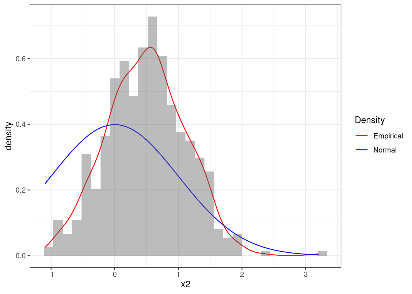

Figure 4.10: Histogram of the sequence x2 together with theoretical pdf of the standard Normal

4.6.1.2 Empirical Cumulative Distribution Function

We have already seen for uniform numbers that we can use the empirical cdf to assess if a sequence of numbers is uniformly distributed. We can use the exact same method for any other distribution.

Figure 4.11 reports the ecdf of the sequence of numbers x1 (in red) together with the theoretical cdf of the standard Normal (in blue). We can see that the two functions match closely and therefore we could assume that the sequence is distributed as a standard Normal.

ggplot(x1, aes(x1)) +
   stat_ecdf(geom = "step",aes(colour = 'Empirical')) +
   stat_function(fun = pnorm,aes(colour = 'Theoretical')) +
   theme_bw() +      
   scale_colour_manual(name = 'Density', values = c('red', 'blue'))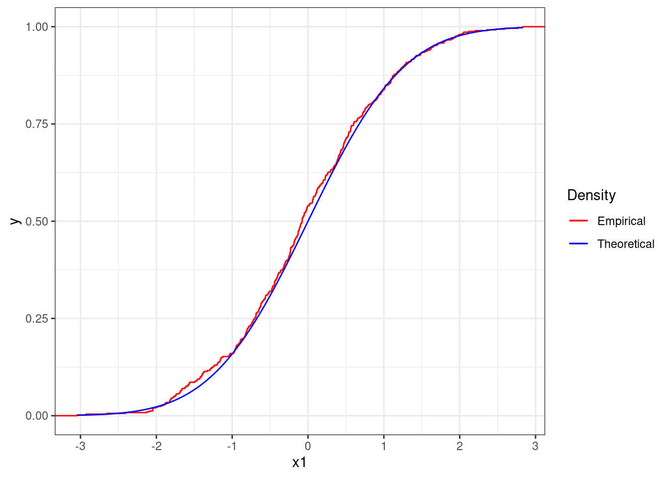

Figure 4.11: Empirical cdf the sequence x1 together with theoretical cdf of the standard Normal

Figure 4.12 reports the same plot but for the sequence x2. The two lines strongly differ and therefore it cannot be assume that the sequence is distributed as a standard Normal.

ggplot(x2, aes(x2)) +
   stat_ecdf(geom = "step",aes(colour = 'Empirical')) +
   stat_function(fun = pnorm,aes(colour = 'Theoretical')) +
   theme_bw() +      
   scale_colour_manual(name = 'Density', values = c('red', 'blue'))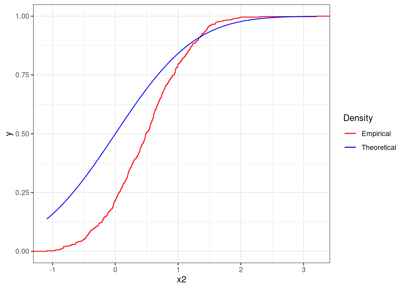

Figure 4.12: Empirical cdf the sequence x2 together with theoretical cdf of the standard Normal

4.6.1.3 QQ-Plot

A third visualization of the distribution of a sequence of numbers is the so called QQ-plot. You may have already seen this when checking if the residuals of a linear regression follow a Normal distribution. But more generally, qq-plots can be used to check if a sequence of numbers is distributed according to any distribution.

We will not the details about how these are constructed but just their interpretation and implementation. Let’s consider Figure 4.13. The plot is composed of a series of points, where each point is associated to a number in our random sequence, and a line, which describes the theoretical distribution we are targeting. The closest the points and the line are, the better the fit to that distribution.

In particular, in Figure 4.13 we are checking if the sequence x1 is distributed according to a standard Normal (represented by the straight line). Since the points are placed almost in a straight line over the theoretical line of the standard Normal, we can assume the sequence to be Normal.

ggplot(x1, aes(sample = x1)) +
   stat_qq(distribution = qnorm) +
   stat_qq_line(distribution = qnorm) +
   theme_bw()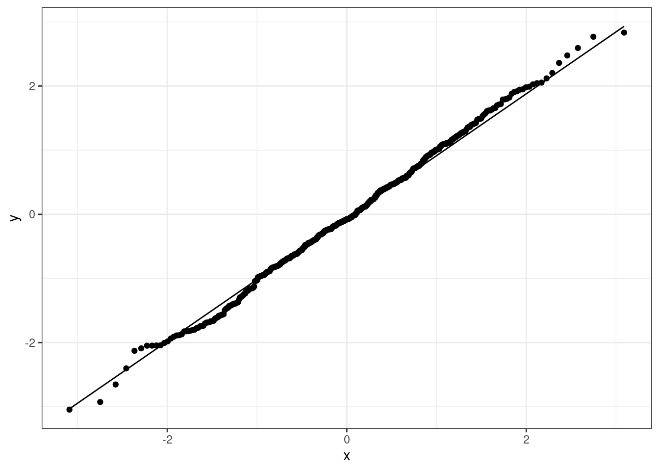

Figure 4.13: QQ-plot for the sequence x1 checking against the standard Normal

Figure 4.14 reports the qq-plot for the sequence x2 to check if the data can be following a standard Normal. We can see that the points do not differ too much from the straight line and in this case we could assume the data to be Normal (notice that the histograms and the cdf strongly suggested that this sequence was not Normal).

ggplot(x2, aes(sample = x2)) +
   stat_qq(distribution = qnorm) +
   stat_qq_line(distribution = qnorm) +
   theme_bw()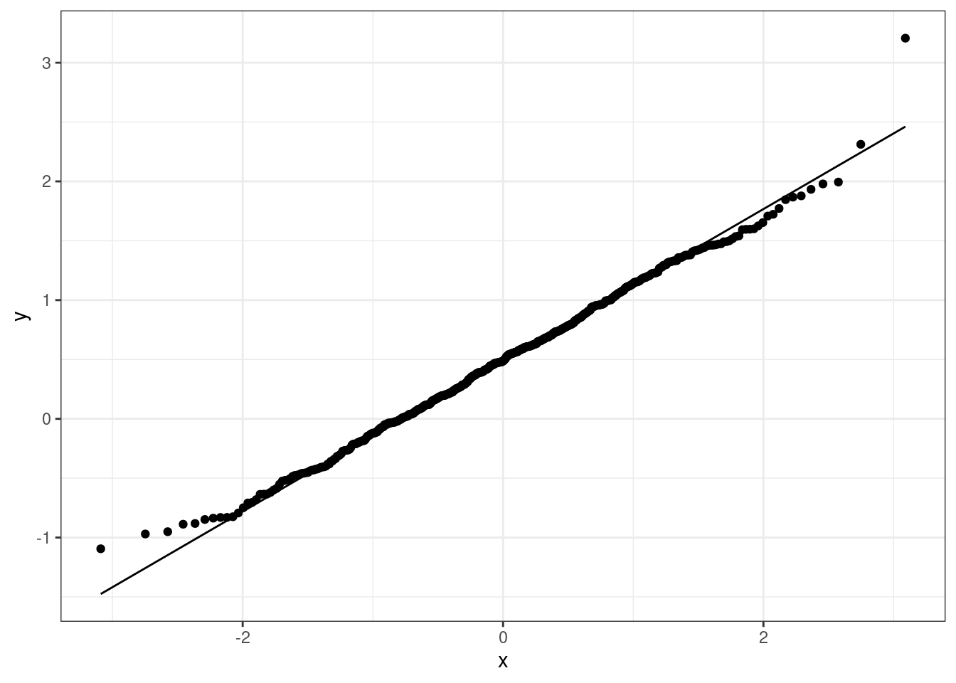

Figure 4.14: QQ-plot for the sequence x2 checking against the standard Normal

Notice that the form of the qq-plot does not only depend on the sequence of numbers we are considering, but also on the distribution we are testing it against. Figure 4.13 reports the qq-plot for the sequence x1 when checked against an Exponential random variable with parameter \(\lambda =3\). Given that the sequence also includes negative numbers, it does not make sense to check if it is distributed as an Exponential (since it can only model non-negative data), but this is just an illustration.

ggplot(x1, aes(sample = x1)) +
   stat_qq(distribution = qexp, dparams = (rate = 3)) +
   stat_qq_line(distribution = qexp, dparams = (rate = 3)) +
   theme_bw()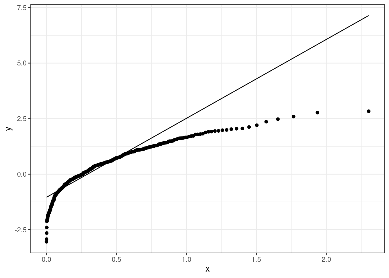

Figure 4.15: QQ-plot for the sequence x1 checking against an Exponential

4.6.1.4 Formal Testing

The above plots are highly informative since they provide insights into the shape of the data distribution, but these are not formal. Again, we can carry out tests of hypothesis to check if data is distributed as a specific random variable, just like we did for the Uniform.

Again, there are many tests one could use, but here we focus only on the Kolmogorov-Smirnov Test which checks how close the empirical and the theoretical cdfs are. It is implemented in the ks.test R function.

Let’s check if the sequences x1 and x2 are distributed as a standard Normal.

ks.test(x1,pnorm)

## 
##  One-sample Kolmogorov-Smirnov test
## 
## data:  x1
## D = 0.041896, p-value = 0.3439
## alternative hypothesis: two-sided

ks.test(x2,pnorm)

## 
##  One-sample Kolmogorov-Smirnov test
## 
## data:  x2
## D = 0.2997, p-value < 2.2e-16
## alternative hypothesis: two-sided

The conclusion is that x1 is distributed as a standard Normal since the p-value of the test is large and for instance bigger than 0.10. On the other hand, the p-value for the Kolmogorov-Smirnov test over the sequence x2 has a very small p-value thus leading us to reject the null hypothesis that the sequence is Normally distributed.

Notice that we can add extra inputs to the function. For instance we can check if x1 is distributed as a Normal with mean = 2 and sd = 2 using:

ks.test(x1, pnorm, mean = 2, sd = 2)

## 
##  One-sample Kolmogorov-Smirnov test
## 
## data:  x1
## D = 0.54604, p-value < 2.2e-16
## alternative hypothesis: two-sided

The p-value is small and therefore we would reject the null hypothesis that the sequence is distributed as a Normal with mean two and standard deviation two.

4.6.2 Testing Independence

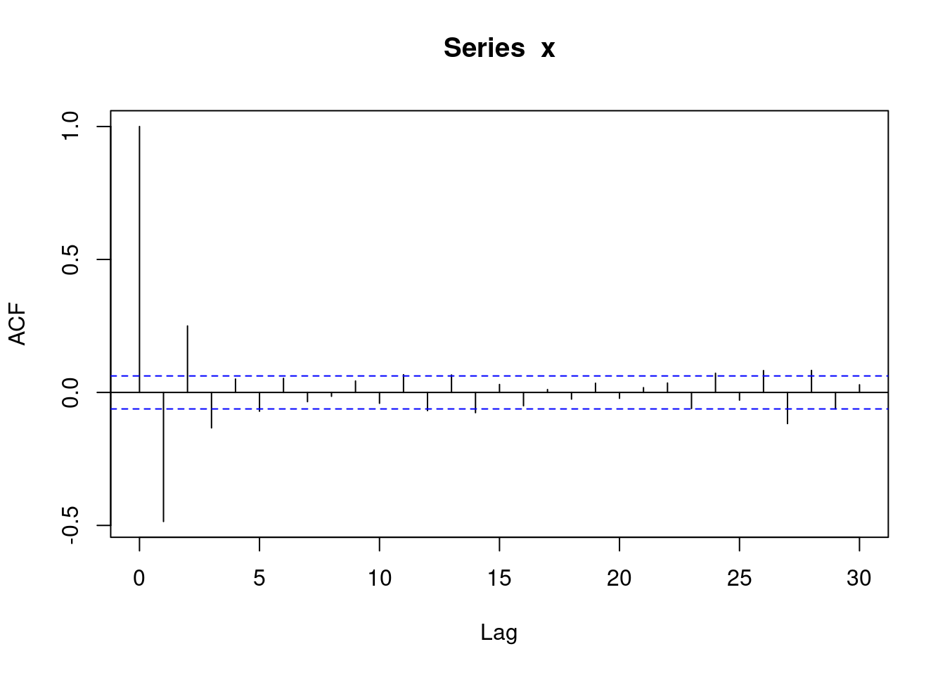
The other step in assessing if a sequence of numbers is pseudo-random is checking if independence holds. We have already learned that one possible way to do this is by computing the auto-correlation function with the R function acf. Let’s compute the auto-correlations of various lags for the sequences x1 and x2, reported in Figure 4.16. We can see that for x2 all bars are within the confidence bands (recall that the first bar for lag \(k=0\) should not be considered). For x1 the bar corresponding to lag 1 is slightly outside the confidence bands, indicating that there may be some dependence.

acf(x1)
acf(x2)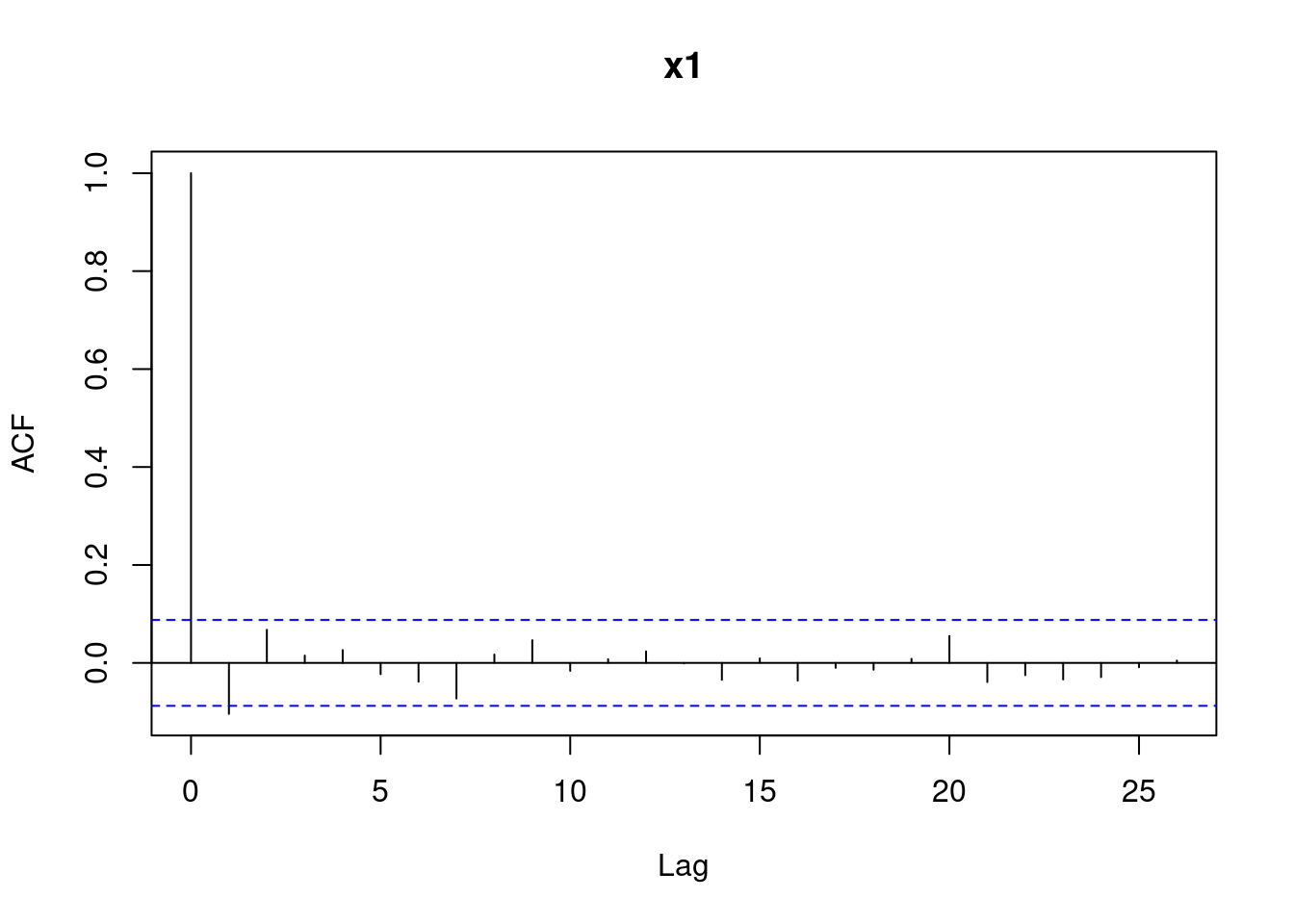

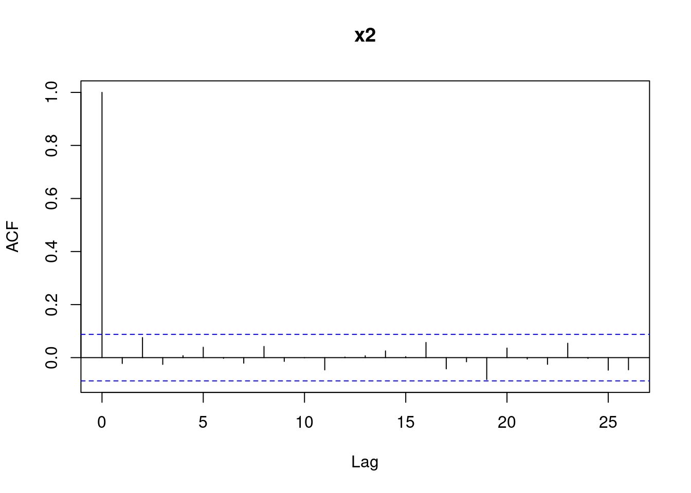
Figure 4.16: Autocorrelations for the sequences x1 and x2.

Let’s run the Box test to assess if the assumption of independence is tenable for both sequences.

Box.test(x1, lag = 5)

## 
##  Box-Pierce test
## 
## data:  x1
## X-squared = 8.4212, df = 5, p-value = 0.1345

Box.test(x2, lag = 5)

## 
##  Box-Pierce test
## 
## data:  x2
## X-squared = 4.2294, df = 5, p-value = 0.5169

In both cases the p-values are larger than 0.10, thus we would not reject the null hypothesis of independence for both sequences. Recall that x1 is distributed as a standard Normal, whilst x2 is not.

For the sequence x1 we observed that one bar was slightly outside the confidence bands: this sometimes happens even when data is actually (pseudo-) random - I created x1 using rnorm. The autocorrelations below are an instance of a case where independence is not tenable since we see that multiple bars are outside the confidence bands.