4.4 Testing Randomness
Now we turn to the following question: given a sequence of numbers \(u_1,\dots,u_N\) how can we test if they are independent realizations of a Uniform random variable between zero and one?
We therefore need to check if the distribution of the numbers is uniform and if they are actually independent.
4.4.1 Testing Uniformity
A simple first method to check if the numbers are uniform is to create an histogram of the data and to see if the histogram is reasonably flat. We already saw how to assess this, but let’s check if runif works well. Simple histograms can be created in R using hist (or if you want you can use ggplot).
set.seed(2021)
u <- runif(5000)
hist(u)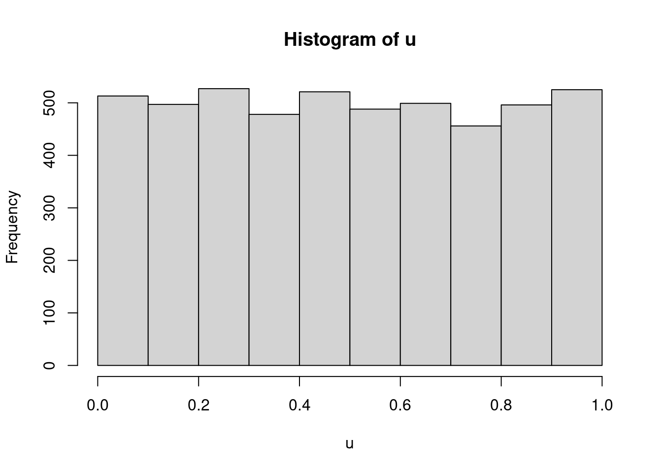
Figure 4.4: Histogram of a sequence of uniform numbers
We can see that the histogram is reasonably flat and therefore the assumption of uniformity seems to hold.
Although the histogram is quite informative, it is not a fairly formal method. We could on the other hand look at tests of hypotheses of this form: \[\begin{align*} H_0: & \;\;u_i \mbox{ is uniform between zero and one, } i=1,2,\dots\\ H_a: & \;\;u_i \mbox{ is not uniform between zero and one, } i=1,2,\dots\\ \end{align*}\]
The null hypothesis is thus that the numbers are indeed uniform, whilst the alternative states that the numbers are not. If we reject the null hypothesis, which happens if the p-value of the test is very small (or smaller than a critical value \(\alpha\) of our choice), then we would believe that the sequence of numbers is not uniform.
There are various ways to carry out such a test, but we will consider here only one: the so-called Kolmogorov-Smirnov Test. We will not give all details of this test, but only its interpretation and implementation.
In order to understand how the test works we need to briefly introduce the concept of empirical cumulative distribution function or ecdf. The ecdf \(\hat{F}\) is the cumulative distribution function computed from a sequence of \(N\) numbers as \[ \hat{F}(t)= \frac{\mbox{numbers in the sequence }\leq t}{N} \]
Let’s consider the following example.
data <- data.frame(u= c(0.1,0.2,0.4,0.8,0.9))
ggplot(data,aes(u)) + stat_ecdf(geom = "step") + theme_bw() + ylab("ECDF")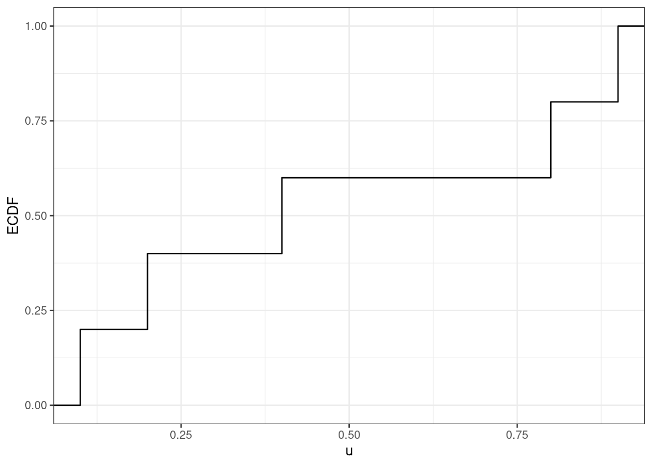
Figure 4.5: Ecdf of a simple sequence of numbers
For instance, since there are 3 numbers out of 5 in the vector u that are less than 0.7, then \(\hat{F}(0.7)=3/5\).
The idea behind the Kolmogorov-Smirnov test is to quantify how similar the ecdf computed from a sequence of data is to the one of the uniform distribution which is represented by a straight line (see Figure 4.2).
As an example consider Figure 4.6. The step functions are computed from two different sequences of numbers between one and zero, whilst the straight line is the cdf of the uniform distribution. By looking at the plots, we would more strongly believe that the sequence in the left plot is uniformly distributed, since the step function is much more closer to the theoretical straight line.
set.seed(2021)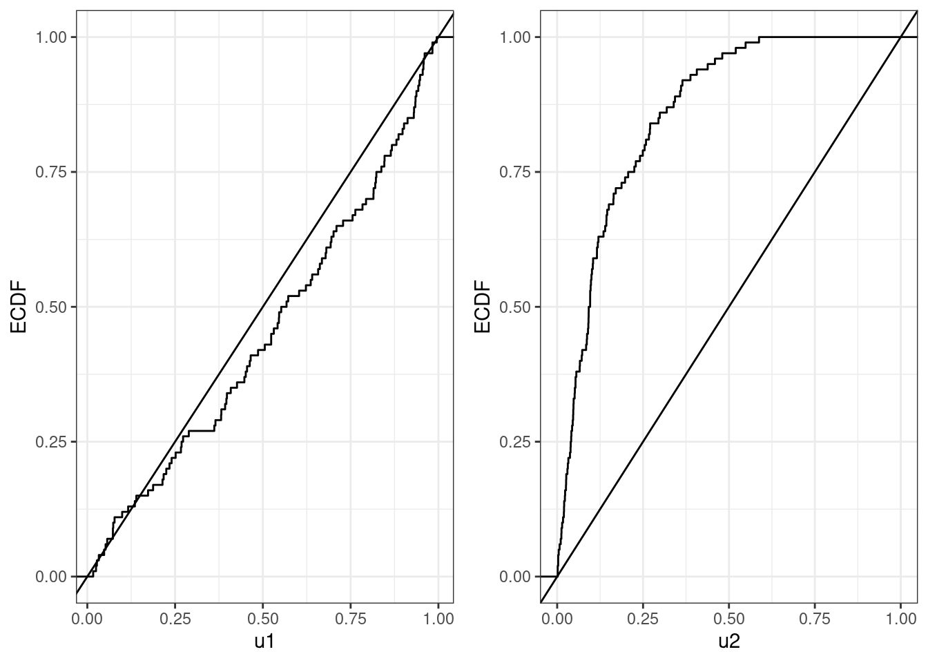
Figure 4.6: Comparison between ecdf and cdf of the uniform for two sequences of numbers
The Kolmogorov-Smirnov test formally embeds this idea of similarity between the ecdf and the cdf of the uniform in a test of hypothesis. The function ks.test implements this test in R. For the two sequences in Figure @ref{fig:Kol} u1 (left plot) and u2 (right plot), the test can be implemented as following:
ks.test(u1,"punif")##
## One-sample Kolmogorov-Smirnov test
##
## data: u1
## D = 0.11499, p-value = 0.142
## alternative hypothesis: two-sidedks.test(u2,"punif")##
## One-sample Kolmogorov-Smirnov test
##
## data: u2
## D = 0.56939, p-value < 2.2e-16
## alternative hypothesis: two-sidedFrom the results that the p-value of the test for the sequence u1 is 0.142 and so we would not reject the null hypothesis that the sequence is uniformly distributed. On the other hand the p-value for the test over the sequence u2 has an extremely small p-value therefore suggesting that we reject the null hypothesis and conclude that the sequence is not uniformly distributed. This confirms our intuition by looking at the plots in Figure 4.6.
4.4.2 Testing Independence
The second requirement that a sequence of pseudo-random numbers must have is independence. We already saw an example of when this might happen: a high number was followed by a low number and vice versa.
We will consider tests of the form:
\[\begin{align*} H_0: & \;\;u_1,\dots,u_N \mbox{ are independent }\\ H_a: & \;\;u_1,\dots,u_N \mbox{ are not independent } \end{align*}\]
So the null hypothesis is that the sequence is of independent numbers against the alternative that they are not. If the p-value of such a test is small we would then reject the null-hypothesis of independence.
In order to devise such a test, we need to come up with a way to quantify how dependent numbers in a sequence are with each other. Again, there are many ways one could do this, but we consider here only one.
You should already be familiar with the idea of correlation: this tells you how to variables are linearly dependent of each other. There is a similar idea which extends in a way correlation to the case when it is computed between a sequence of numbers and itself, which is called autocorrelation. We will not give the details about this, but just the interpretation (you will learn a lot more about this in Time Series).
Let’s briefly recall the idea behind correlation. Suppose you have two sequences of numbers \(u_1,\dots,u_N\) and \(w_1,\dots,w_N\). To compute the correlation you would look at the pairs \((u_1,w_1),(u_2,w_2),\dots, (u_N,w_N)\) and assess how related the numbers within a pair \((u_i,w_i)\) are. Correlation, which is a number between -1 and 1, assesses how related the sequences are: the closer the number is to one in absolute value, the stronger the relationship.
Now however we have just one sequence of numbers \(u_1,\dots,u_N\). So for instance we could look at pairs \((u_1,u_2), (u_2,u_3), \dots, (u_{N-1},u_{N})\) which consider two consecutive numbers and compute their correlation. Similarly we could compute the correlation between \((u_1,u_{1+k}), (u_2,u_{2+k}),\dots, (u_{N-k},u_N)\) between each number in the sequence and the one k-positions ahead. This is what we call autocorrelation of lag k.
If autocorrelations of various lags are close to zero, this gives an indication that the data is independent. If on the other hand, the autocorrelation at some lags is large, then there is an indication of dependence in the sequence of random numbers. Autocorrelations are computed and plotted in R using acf and reported in Figure 4.7.
set.seed(2021)
u1 <- runif(200)
acf(u1)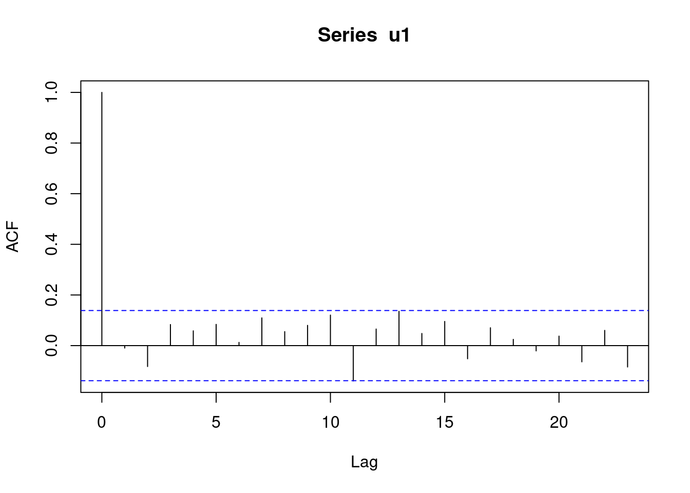
Figure 4.7: Autocorrelations for a sequence of random uniform numbers
The bars in Figure 4.7 are the autocorrelations at various lags, whilst the dashed blue lines are confidence bands: if a bar is within the bands it means that we cannot reject the hypothesis that the autocorrelation of the associated lag is equal to zero. Notice that the first bar is lag 0: it computes the correlation for the sample \((u_1,u_1),(u_2,u_2),\dots,(u_N,u_N)\) and therefore it is always equal to one. You should never worry about this bar. Since all the bars are within the confidence bands, we believe that all autocorrelations are not different from zero and consequently that the data is independent (it was indeed generated using `runif``).
Figure 4.8 reports the autocorrelations of a sequence of numbers which is not independent. Although the histogram shows that the data is uniformly distributed, we would not believe that the sequence is of independent numbers since autocorrelations are very large and outside the bands.
u2 <- rep(1:10,each = 4,times = 10)/10 + rnorm(400,0,0.02)
u2 <- (u2 - min(u2))/(max(u2)-min(u2))
par(mfrow=c(1,2))
hist(u2)
acf(u2)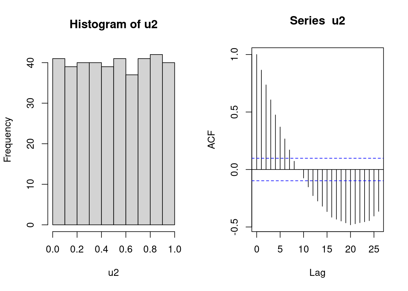
Figure 4.8: Histogram and autocorrelations of a sequence of uniform numbers which are not independent
A test of hypothesis for independence can be created by checking if any of the autocorrelations up to a specific lag are different from zero. This is implemented in the function Box.test in R. The first input is the sequence of numbers to consider, the second is the largest lag we want to consider. Let’s compute it for the two sequences u1 and u2 above.
Box.test(u1, lag = 5)##
## Box-Pierce test
##
## data: u1
## X-squared = 4.8518, df = 5, p-value = 0.4342Box.test(u2, lag = 5)##
## Box-Pierce test
##
## data: u2
## X-squared = 807.1, df = 5, p-value < 2.2e-16Here we chose a lag up to 5 (it is usually not useful to consider larger lags). The test confirms our observations of the autocorrelations. For the sequence u1 generated with runif the test has a high p-value and therefore we cannot reject the hypothesis of independence. For the second sequence u2 which had very large autocorrelations the p-value is very small and therefore we reject the hypothesis of independence.