3.5 Notable Discrete Variables
In the previous section we gave a generic definition of discrete random variables and discussed the conditions that a pmf must obey. We considered the example of a biased dice and constructed a pmf for that specific example.
There are situations that often happen in practice: for instance the case of experiments with binary outcomes. For such cases random variables with specific pmfs are given a name and their properties are well known and studied.
In this section we will consider three such distributions: Bernoulli, Binomial and Poisson.
3.5.1 Bernoulli Distribution
Consider an experiment or a real-world system where there can only be two outcomes:
a toss of a coin: heads or tails;
the result of a COVID test: positive or negative;
the status of a machine: broken or working;
By default one outcome happens with some probability, that we denote as \(p\in [0,1]\) and the other with probability \(1-p\).
Such a situation is in general modeled using the so-called Bernoulli distribution with parameter \(p\). One outcome is associated to the number 1 (usually referred to as sucess) and the other is associated to the number 0 (usually referred to as failure). So \(P(X=1)=p(1)=p\) and \(P(X=0)=p(0)=1-p\).
The above pmf can be more coincisely written as \[ p(x)=\left\{ \begin{array}{ll} p^x(1-p)^{1-x}, & x=0,1\\ 0, & \mbox{otherwise} \end{array} \right. \] The mean and variance of the Bernoulli distribution can be easily computed as \[ E(X)=0\cdot(1-p)+ 1\cdotp=p, \] and \[ V(X)=(0-p)^2(1-p)+(1-p)^2p=p^2(1-p)+(1-p)^2p=\cdots = p(1-p) \]
Figure 3.3 reports the pmf and the cdf of a Bernoulli random variable with parameter 0.3.
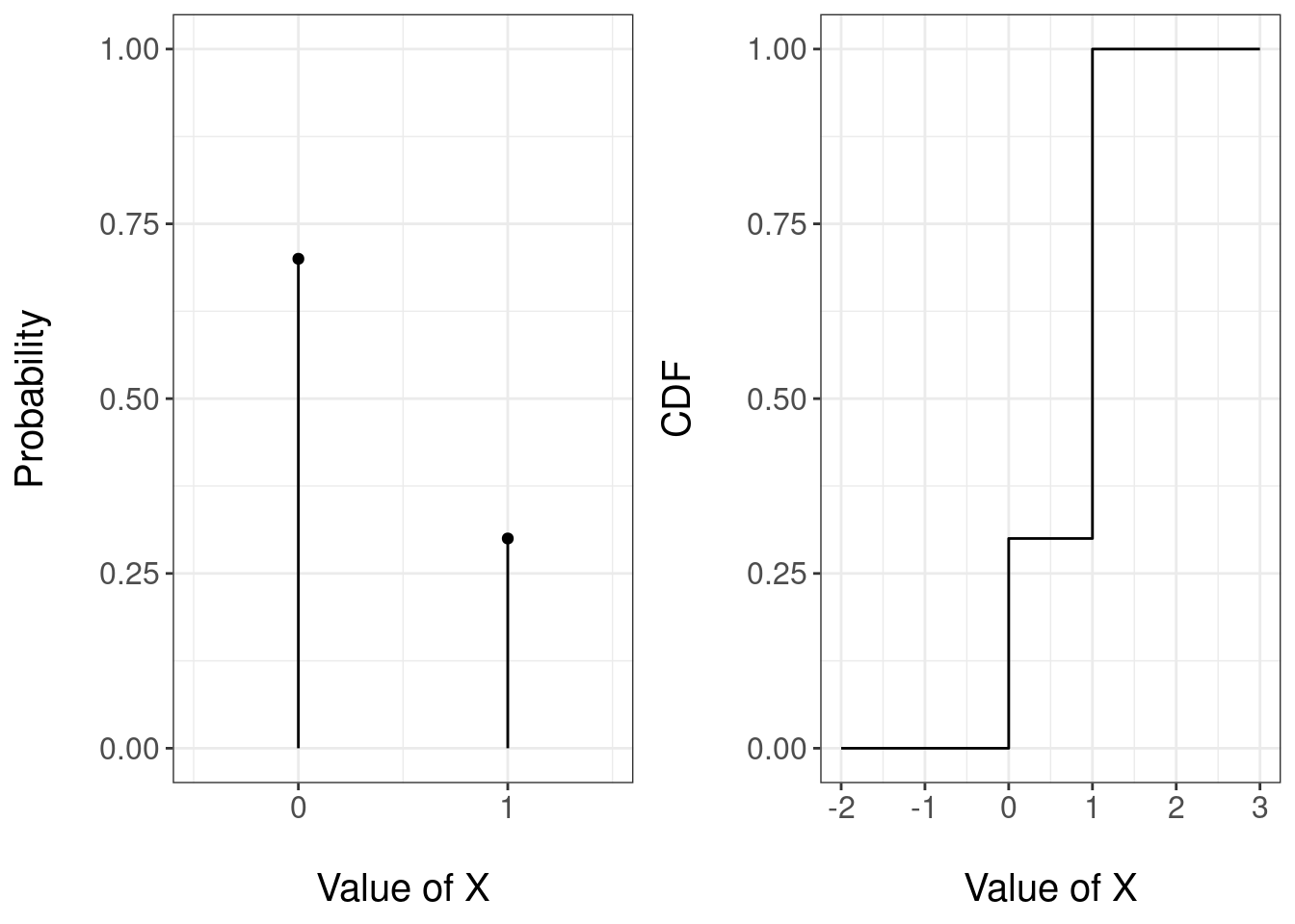
Figure 3.3: PMF (left) and CDF (right) of a Bernoulli random variable with parameter 0.3
R doesn’t provides a specific method for the Bernoulli distribution, but as we will see in the next section, this is a specific case of the binomial experiment, so we will use the binomial method for working with the Bernoulli distribution in R. We will explain this function below, for now let’s see a couple examples of the Bernoulli \(Ber(p=0.25)\) distribution in R
dbinom(0,size=1,prob=0.25) # probability of failure## [1] 0.75dbinom(1,size=1,prob=0.25) # probability of success## [1] 0.25rbinom(n=20,size = 1,prob=0.25) # generating 20 random numbers from a Bernoulli distribution with p = 0.25## [1] 0 0 0 0 0 1 0 0 0 0 1 0 0 1 0 0 0 1 1 03.5.2 Binomial Distribution
The Bernoulli random variable is actually a very special case of the so-called Binomial random variable. Consider experiments of the type discussed for Bernoullis: coin tosses, COVID tests etc. Now suppose that instead of having just one trial, each of these experiments are repeated multiple times. Consider the following assumptions:
each experiment is repeated \(n\) times;
each time there is a probability of success \(p\);
the outcome of each experiment is independent of the others.
Let’s think of tossing a coin \(n\) times. Then we would expect that the probability of showing heads is the same for all tosses and that the result of previous tosses does not affect others. So this situation appears to meet the above assumptions and can be modeled by what we call a Binomial random variable.
Formally, the random variable \(X\) is a Binomial random variable with parameters \(n\) and \(p\) if it denotes the number of successes of \(n\) independent Bernoulli random variables, all with parameter \(p\).
The pmf of a Binomial random variable with parameters \(n\) and \(p\) can be written as: \[ p(x)=\left\{ \begin{array}{ll} \binom{n}{x}p^{x}(1-p)^{n-x}, & x = 0,1,\dots,n\\ 0, & \mbox{otherwise} \end{array} \right. \] Let’s try and understand the formula by looking term by term.
if \(X=x\) there are \(x\) successes and each success has probability \(p\) - so \(p^x\) counts the overall probability of successes
if \(X=x\) there are \(n-x\) failures and each failure has probability \(1-p\) - so \((1-p)^{n-x}\) counts the overall probability of failures
failures and successes can appear according to many orders. To see this, suppose that \(x=1\): there is only one success out of \(n\) trials. This could have been the first attempt, the second attempt or the \(n\)-th attempt. The term \(\binom{n}{x}\) counts all possible ways the outcome \(x\) could have happened.
The Bernoulli distribution can be seen as a special case of the Binomial where the parameter \(n\) is fixed to 1.
We will not show why this is the case but the expectation and the variance of the Binomial random variable with parameters \(n\) and \(p\) can be derived as \[ E(X)=np, \hspace{2cm} V(X)=np(1-p) \] The formulae for the Bernoulli can be retrieved by setting \(n=1\).
Figure 3.4 shows the pmf of two Binomial distributions both with parameter \(n=10\) and with \(p=0.3\) (left) and \(p=0.8\). For the case \(p=0.3\) we can see that it is more likely that there are a small number of successes, whilst for \(p=0.8\) a large number of successes is more likely.
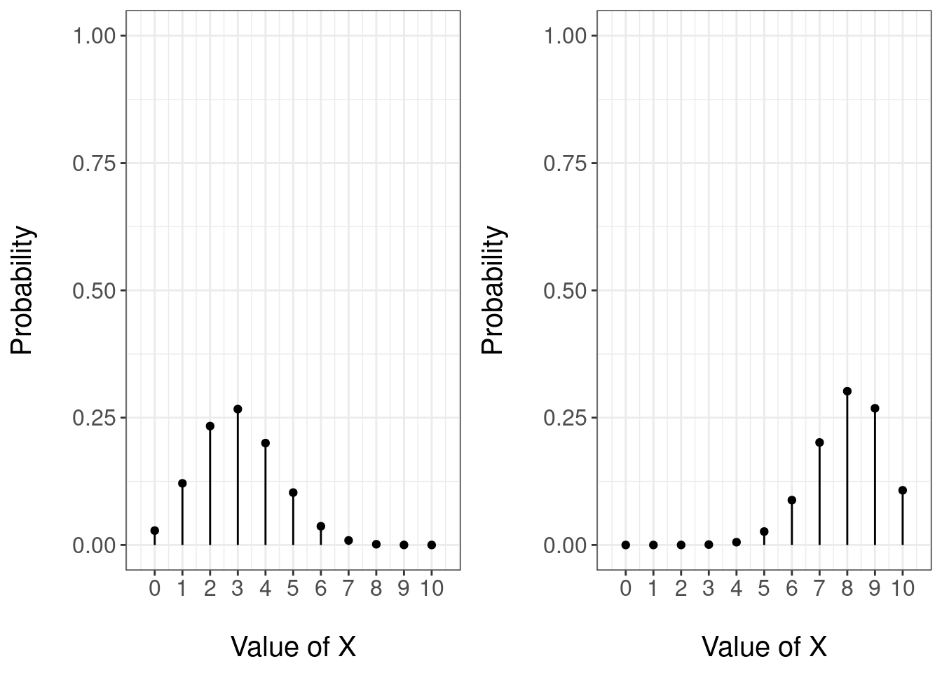
Figure 3.4: PMF of a Binomial random variable with parameters n = 10 and theta = 0.3 (left) and theta = 0.8 (right)
R provides a straightforward implementation of the Binomial distribution through the functions dbinom for the pmf and pbinom for the cdf. They require three arguments:
first argument is the value at which to compute the pmf or the cdf;
sizeis the parameter \(n\) of the Binomial;probis the parameter \(p\) of the Binomial.
So for instance
dbinom(3, size = 10, prob = 0.5)## [1] 0.1171875returns \(P(X=3)=p(3)\) for a Binomial random variable with parameter \(n=10\) and \(p = 0.5\).
Similarly,
pbinom(8, size = 20, prob = 0.2)## [1] 0.9900182returns \(P(X\leq 8) = F(8)\) for a Binomial random variable with parameter \(n=20\) and \(p = 0.2\).
R also provides a method for generating pseudo-random numbers using a binomial distribution through the function rbinom. This function will require three arguments:
nis the parameter for specifying the number of pseudo-random numbers we want to generate;sizeis the parameter \(n\) of the Binomial;probis the parameter \(p\) of the Binomial.
Example 3.2 Example The below example would be equivalent to repeating 100 times the experiment of tossing a coin 20 times and counting the number of heads.
rbinom(100,size = 20,prob=0.5)## [1] 8 8 11 11 8 10 12 9 10 5 12 9 10 7 12 10 9 8 11 12 11 10 13 5 10
## [26] 6 9 10 15 11 11 13 8 8 8 15 8 11 9 13 12 9 15 12 12 11 9 12 12 9
## [51] 9 15 12 7 9 9 13 10 8 9 9 10 11 10 7 9 6 12 11 10 9 10 9 9 11
## [76] 10 6 12 12 9 7 12 9 10 13 14 10 11 11 8 9 16 11 11 10 13 10 10 10 103.5.3 Geometric distribution
We’ve all played a coin toss until we get the first head, or even throwing a ball into a basketball hoop until we get the first one in. From another point of view we can also try to model the number of times we flip a switch and the bulb lights up until it fails, or the number of times an ATM gives us money until it fails.
The modelling of this kind of problems is achieved with the so called Geometric Distribution.
- Let’s repeat a Bernoulli experiment, of \(p\) parameter, independently until we get the first success.
- Let \(X\) be the random variable that counts the number of failures before the first success. For example, if we have had \(x\) failures, it will be a sequence of \(x\) failures culminated with a success. More specifically
\[ P(\overbrace{FFF\ldots F}^{x}S)=P(F)^{x}\cdot P(S)=(1-p)^{x}\cdot p=q^{x}\cdot p. \]
Its probability function is
\[ P_X(x)=P(X=x)=\left\{\begin{array}{ll} (1-p)^{x}\cdot p & \mbox{ if } x=0,1,2,\ldots\\ 0 &\mbox{ otherwise} \end{array}\right.. \]
The random variable defined above is said to follow a geometric distribution of \(p\) parameter. We will denote it by \(Ge(p)\). Its domain is \(D_X=\{0,1,2,\ldots\}\).
Now imagine that we want to calculate P(\(X\leq 3\)). By the property of the probability of the complementary event we have that
\[ P(X\leq 3 )=1-P(X> 3)=1-P(X\geq 4) \]
In fact, the \(X\leq 3\) complementary tells us that we have failed more than three times until we get the first success, that is, we have failed 4 or more times. We can symbolize this event in the following way:
\[ \{X>3\}=\{X\geq 4\}= \{FFFF\} \]
Now, since the attempts are independent, we have that:
\[\begin{align} P(X>3) & = & P(\{FFFF\})= P(F)\cdot P(F)\cdot P(F)\cdot P(F)\\ &=& (1-p)\cdot (1-p)\cdot (1-p)\cdot (1-p)= (1-p)^{3+1}\\ &=&(1-p)^{4} \end{align}\]
The value of the distribution function of \(X\) in \(x=3\) will be:
\[ F_X(3)=P(X\leq 3)=1-P(X>3)=1-(1-p)^{3+1}. \]
Generalizing the result before any positive integer \(k=0,1,2,\ldots\), we have that:
\[ F_X(k)=P(X\leq k)=1-(1-p)^{k+1},\mbox{ if } k=0,1,2,\ldots \]
In general, we’ll have that: \[ F_X(x)=P(X\leq x)= \left\{\begin{array}{ll} 0, & \mbox{ if } x<0,\\ 1- (1-p), & \mbox{ if } k=0\leq x <1,\\ 1- (1-p)^2, & \mbox{ if } k=1\leq x <2,\\ 1- (1-p)^3, & \mbox{ if } k=2\leq x <3,\\ 1- (1-p)^{k+1}, & \mbox{ si } \left\{ \begin{array}{l}k\leq x< k+1,\\\mbox{for } k=0,1,2,\ldots\end{array} \right.\end{array}\right. \]
More compactly, we’ll have that: \[ F_X(x)=P(X\leq x)= \left\{\begin{array}{ll} 0, & \mbox{ if } x<0,\\ 1- (1-p)^{k+1}, & \mbox{ if } \left\{ \begin{array}{l}k\leq x< k+1,\\\mbox{for } k=0,1,2,\ldots\end{array} \right.\end{array} \right. \]
Notice that the limit of the distribution function is: \[ \displaystyle\lim_{k\to +\infty } F_X(k)=\lim_{k\to +\infty } 1-(1-p)^{k+1}= 1, \]
We will not show here the calculation of the expectation and variance of a geometric random variable. They can be derived as:
\[\begin{align} E(X)= \frac{1-p}{p}, \\ Var(X) = \frac{1-p}{p^2} \end{align}\]
And its standard desviation is:
\[ \sqrt{Var(X)}=\sqrt{\frac{1-p}{p^2}} \]
Another interpretation of the geometric random variable is using the number of attempts rather than the number of failures. Let’s say we’re only interested in the number of attempts to get the first success. If we define \(Y\)= number of attempts to get the first success Then \(Y=X+1\) where \(X\equiv Ge(p)\). Its domain is \(D_Y=\{1,2,\ldots\}\). The average increases in one attempt due to success \(E(Y)=E(X+1)=E(X)+1=\frac{1-p}{p}+1=\frac1{p}\). The variance is the same \(Var(Y)=Var(X+1)=Var(X)=\frac{1-p}{p^2}\).
\(Ge(p)\) starting in 0 is the experiment to calculate the probability of having a specific number of attempts to obtain the first success
R provides a method for performing calculations with a geometric random variable. The dgeom and pgeom functions will have the next arguments:
xwill take the value of the geometric random variable we want to evaluateprobis the probability of success in each of the attempts
Let’s see some examples for the geometric distribution \(Ge(p=0.25)\).
\(P(X=0)=(1-0.25)^0\cdot 0.25^1=0.25\)
dgeom(x = 0, prob=0.25)## [1] 0.25\(P(X\leq 0)=1- (1-0.25)^{0+1}=1-0.75=0.25\)
pgeom(0,prob=0.25)## [1] 0.25\(P(X\leq 4)=1-(1-0.25)^{4+1}=1-0.75^5 = 0.76\)
pgeom(4,prob=0.25)## [1] 0.7626953R also provides a method for generating pseudo-random numbers using a geometric distribution. The parameters of this function are:
nis the amount of pseudo-random numebers we want to generateprobis the probability of success in each of the attempts
A random sample of size 25 of a \(Ge(0.25)\) can be generated as:
rgeom(n=25,prob=0.25)## [1] 0 1 2 11 0 6 7 13 5 2 5 5 0 1 2 2 0 0 0 0 9 1 2 3 0Figure 3.5 shows the PMF and CDF of a Geometric distribution with parameter \(n=30\) and with \(p=0.25\).
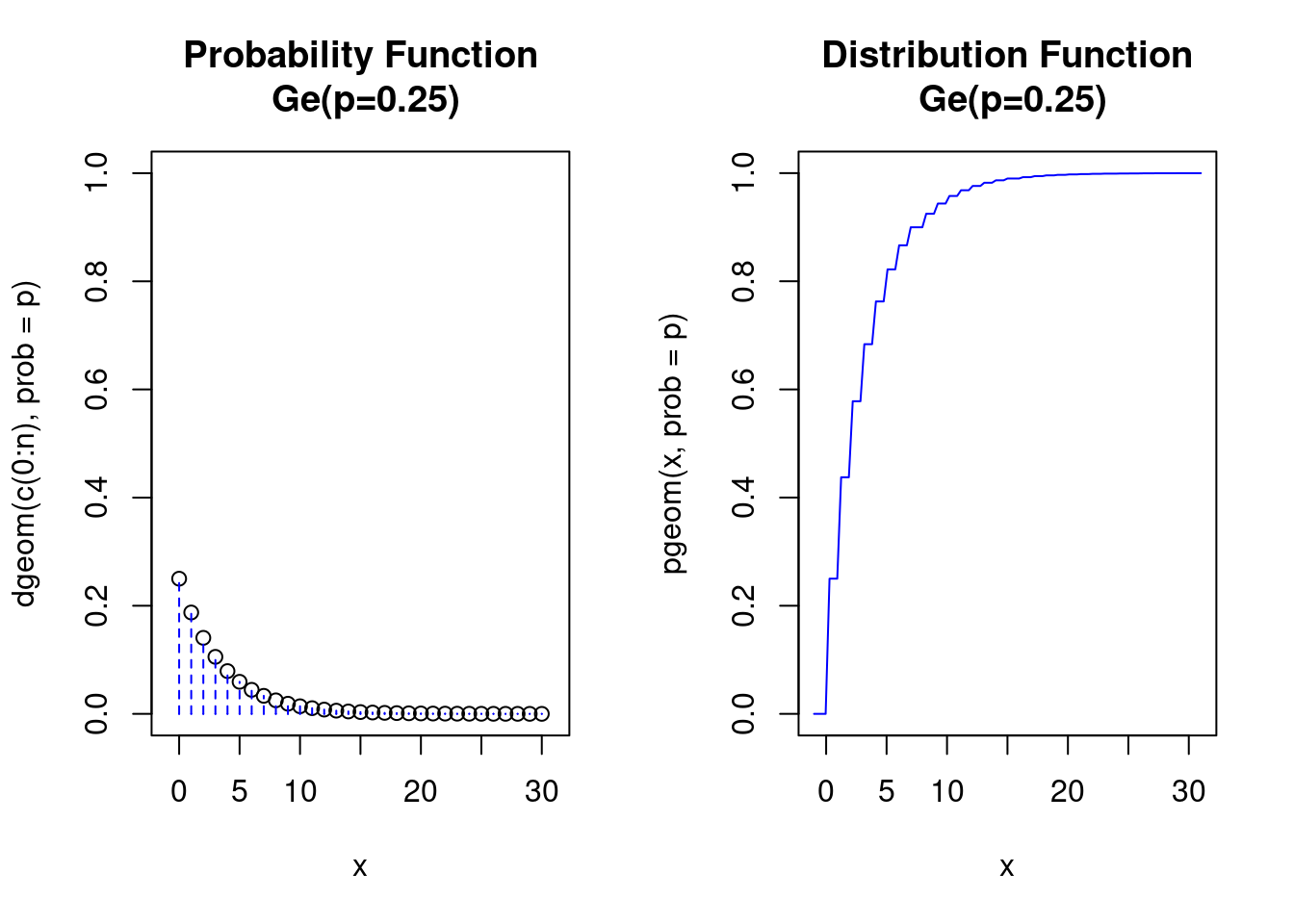
Figure 3.5: PMF and CDF of a Geometric random variable with parameters n = 30 and p = 0.25
3.5.4 Poisson Distribution
The last class of discrete random variables we discuss is the so-called Poisson distribution. Whilst for Bernoulli and Binomial we had an interpretation of why the pmf took its specific form by associating it to independent binary experiments each with an equal probability of success, for the Poisson there is no such an interpretation.
A discrete random variable \(X\) has a Poisson distribution with parameter \(\lambda\) if its pmf is \[ p(x)=\left\{ \begin{array}{ll} \frac{e^{-\lambda}\lambda^x}{x!}, & x = 0,1,2,3,\dots\\ 0, & \mbox{otherwise} \end{array} \right. \] where \(\lambda > 0\).
So the sample space of a Poisson random variable is the set of all non-negative integers.
One important characteristic of the Poisson distribution is that its mean and variance are equal to the parameter \(\lambda\), that is \[ E(X)= V(X) = \lambda. \]
Figure 3.6 gives an illustration of the form of the pmf of the Poisson distribution for two parameter choices: \(\lambda=1\) (left) and \(\lambda = 4\) (right). The x-axis is shown until \(x=10\) but recall that the Poisson is defined over all non-negative integers. For the case \(\lambda=1\) we can see that the outcomes 0 and 1 have the largest probability - recall that \(E(X)=0\). For the case \(\lambda = 4\) the outcomes \(x = 2,3,4,5\) have the largest probability.
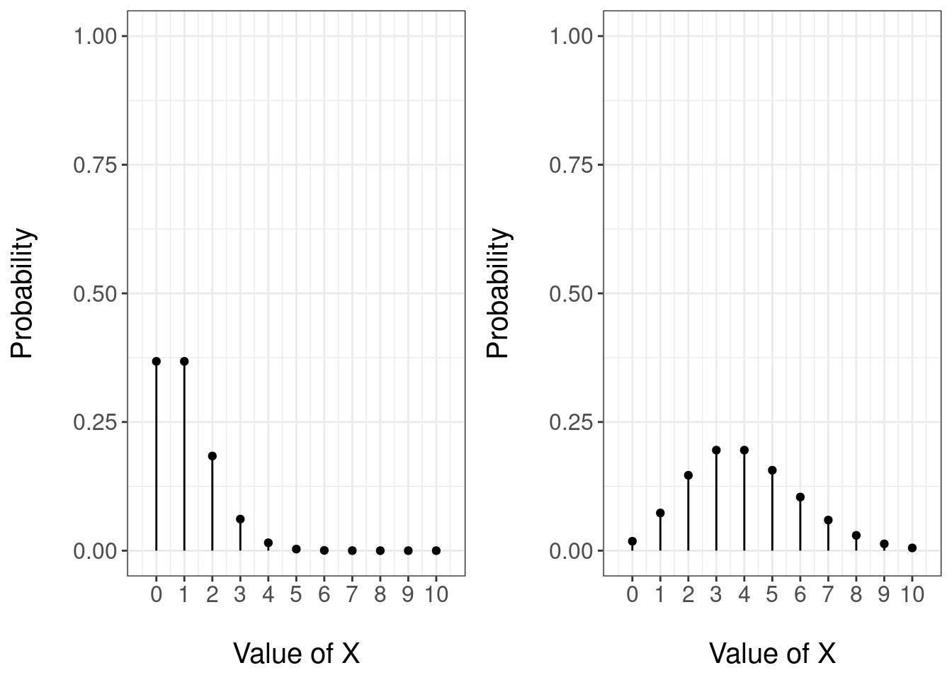
Figure 3.6: PMF of a Poisson random variable with parameter 1 (left) and 4 (right)
The interesting thing about Poisson variables is that we can modify (if the model allows it) the time interval \((0,t]\) in which we count the events. Of course, this doesn’t necessarily have to be possible. But in general if the variable is poisson in \((0,t]\) it will be also in any sub-interval \((0,t']\) for all \(t'\) such that \(0<t'<t\). So we will be able to define a series of variables \(X_t\) of distribution \(Po(t)\).
R provides a straightforward implementation of the Poisson distribution through the functions dpois for the pmf and ppois for the cdf. They require three arguments:
first argument is the value at which to compute the pmf or the cdf;
lambdais the parameter \(\lambda\) of the Poisson;
So for instance
dpois(3, lambda = 1)## [1] 0.06131324returns \(P(X=3)=p(3)\) for a Poisson random variable with parameter \(\lambda = 1\).
Similarly,
ppois(8, lambda = 4)## [1] 0.9786366returns \(P(X\leq 8) = F(8)\) for a Poisson random variable with parameter \(\lambda = 4\).
We can also generate pseudo-random numbers from a poisson distribution using the rpois method. This method has two arguments in r:
namount of pseudo-random numberslambdais the expectation for a specific time interval
This way,
rpois(n=100,lambda = 3)## [1] 1 2 2 3 2 5 3 2 3 7 2 4 7 1 1 3 3 6 1 1 2 3 2 3 1 2 0 4 2 2 1 1 5 4 2 4 1
## [38] 3 2 1 2 3 2 3 4 3 3 4 4 2 1 4 5 1 2 3 3 1 1 3 0 3 1 2 4 2 6 3 5 3 0 2 1 1
## [75] 6 2 7 4 0 2 2 4 1 3 4 3 5 2 2 1 4 2 4 5 4 4 2 3 1 6Returns a sequence of 100 observations for a Poisson distribution of = 3.
3.5.5 Some Examples
We next consider two examples to see in practice the use of the Binomial and Poisson distributions.
3.5.5.1 Probability of Marriage
A recent survey indicated that 82% of single women aged 25 years old will be married in their lifetime. Compute
the probability of at most 3 women will be married in a sample of 20;
the probability of at least 90 women will be married in sample of 100;
the probability of two or three women in a sample of 20 will never be married.
The above situation can be modeled by a Binomial random variable where the parameter \(n\) depends on the question and \(p = 0.82\).
The first question requires us to compute \(P(X\leq 3)= F(3)\) where \(X\) is Binomial with parameters \(n=20\) and \(p =0.82\). Using R
pbinom(3, size = 10, prob = 0.82)## [1] 0.0004400767The second question requires us to compute \(P(X\geq 90)\) where \(X\) is a Binomial random variable with parameters \(n=100\) and \(p = 0.82\). Notice that \[ P(X\geq 90) = 1 - P(X< 90) = 1 - P(X\leq 89) = 1 - F(89). \] Using R
1 - pbinom(89, size = 100, prob = 0.82)## [1] 0.02003866For the third question, notice that saying two women out of 20 will never be married is equal to 18 out of 20 will be married. Therefore we need to compute \(P(X=17) + P(X=18)= p(17) + p(18)\) where \(X\) is a Binomial random variable with parameters \(n=20\) and \(p = 0.82\). Using R
sum(dbinom(17:18, size = 20, prob = 0.82))## [1] 0.40076313.5.5.2 The Bad Stuntman
A stuntman injures himself an average of three times a year. Use the Poisson probability formula to calculate the probability that he will be injured:
4 times a year
Less than twice this year.
More than three times this year.
The above situation can be modeled as a Poisson distribution \(X\) with parameter \(\lambda = 3\).
The first question requires us to compute \(P(X=4)\) which using R can be computed as
dpois(4, lambda =3)## [1] 0.1680314The second question requires us to compute \(P(X<2) = P(X=0)+P(X=1)= F(1)\) which using R can be computed as
ppois(1,lambda=3)## [1] 0.1991483The third question requires us to compute \(P(X>3) = 1 - P(X\leq 2) = 1 - F(2)\) which using R can be computed as
1 - ppois(2, lambda = 3)## [1] 0.5768099