4.1 Properties of Random Numbers

The first step to simulate numbers from a distribution is to be able to independently simulate random numbers \(u_1,u_2,\dots,u_N\) from a continuous uniform distribution between zero and one. From the previous chapter, you should remember that such a random variables has pdf \[ f(x)=\left\{ \begin{array}{ll} 1, & 0\leq x \leq 1\\ 0, &\mbox{otherwise} \end{array} \right. \] and cdf \[ F(x)=\left\{ \begin{array}{ll} 0, & x<0\\ x, & 0\leq x \leq 1\\ 1, &\mbox{otherwise} \end{array} \right. \] These two are plotted in Figure 4.2.

x <- c(seq(-1,0,0.01),seq(0,1,0.01),seq(1,2,0.01))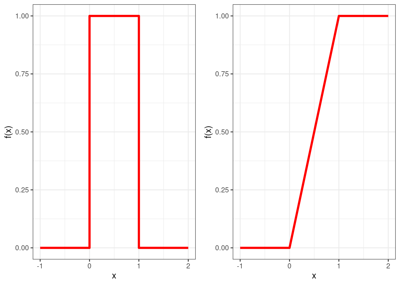

Figure 4.2: Pdf (left) and cdf (right) of the continuous uniform between zero and one.

Its expectation is 1/2 and its variance is 1/12.

This implies that if we were to divide the interval \([0,1]\) into \(n\) sub-intervals of equal length, then we would expect in each interval to have \(N/n\) observations, where \(N\) is the total number of observations.

Figure 4.3 shows the histograms of two sequences of numbers between zero and one: whilst the one on the left resembles the pdf of a uniform distribution, the one on the right clearly does not (it is far from being flat) and therefore it is hard to believe that such numbers follow a uniform distribution.

p <- ggplot(data.frame(x1=runif(10000)), aes(x=x1))+
   geom_histogram(aes(y=..density..),binwidth=0.1,center = 0.05, colour="black", fill="white")  + theme_bw()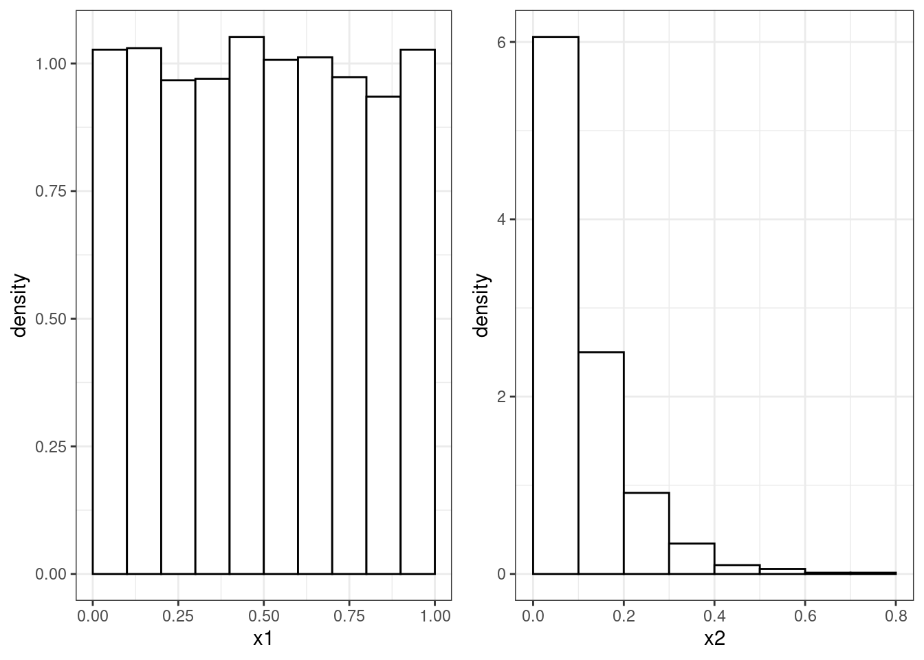 

Figure 4.3: Histograms from two sequences of numbers between zero and one.

The second requirement the numbers \(u_1,\dots,u_N\) need to respect is independence. This means that the probability of observing a value in a particular sub-interval of \((0,1)\) is independent of the previous values drawn.

Consider the following sequence of numbers: \[ \begin{array}{cccccccccc} 0.25 & 0.72 & 0.18 & 0.63 & 0.49 & 0.88 & 0.23 & 0.78 & 0.02 & 0.52 \end{array} \] We can notice that numbers below and above 0.5 are alternating in the sequence. We would therefore believe that after a number less than 0.5 it is much more likely to observe a number above it. This breaks the assumption of independence.