Chapter 4 Random Number Generation

At the hearth of any simulation model there is the capability of creating numbers that mimic those we would expect in real life. In simulation and modeling we will assume that specific processes will be distributed according to a specific random variable. For instance we will assume that an employee in a donut shop takes a random time to serve customers distributed according to a Normal random variable with mean \(\mu\) and variance \(\sigma^2\). In order to then carry out a simulation the computer will need to generate random serving times. This corresponds to simulating number that are distributed according to a specific distribution.

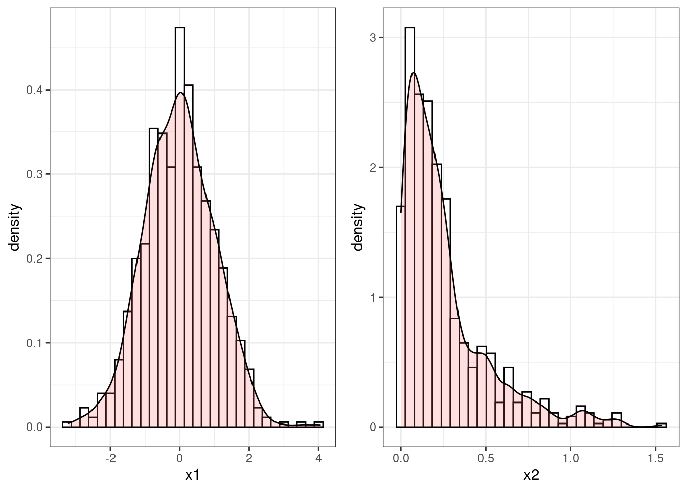
Let’s consider an example. Suppose you managed to generate two sequences of numbers, say x1 and x2. Your objective is to simulate numbers from a Normal distribution. The histograms of the two sequences are reported in Figure 4.1 together with the estimated shape of the density. Clearly the sequence x1 could be following a Normal distribution, since it is bell-shaped and reasonably symmetric. On the other hand, the sequence x2 is not symmetric at all and does not resembles the density of a Normal.

p <- ggplot(data.frame(x1=rnorm(700)), aes(x=x1))+
   geom_histogram(aes(y=..density..), colour="black", fill="white")+
 geom_density(alpha=.2, fill="#FF6666")  + theme_bw() 

## `stat_bin()` using `bins = 30`. Pick better value with `binwidth`.

Figure 4.1: Histograms of two sequences of randomly generated numbers

In this chapter we will learn how to characterize randomness in a computer and how to generate numbers that appear to be random realizations of a specific random variable. We will also learn how to check if a sequence of values can be a random realization from a specific random variable.