6.3 The taxi problem (comparing estimators)
Finally, we will see a case in which we want to compare two different estimators. Imagine that a person is walking through the streets of a city and notices the following numbers of 5 taxis that pass by: 34,100,65,81,120. Can he/she make an intelligent guess at the number of taxis in the city?: Is a problem of statistical inference where population is collection of taxis driven in city and one wishes to know unknown number of taxis \(N\).
Assume taxis are numbered from \(1\) to \(N\), each equally likely to be observed and consider two possible estimates:
- The largest taxi number observed
- Twice the sample mean.
Which is a better estimator of the number of taxis \(N\)? We will compare these two estimators using a Monte Carlo Simulation:
- Simulate taxi numbers from a uniform distribution with a known number of taxis \(N\) and compute the two estimates.
- Repeat many times and obtain two empirical sampling distributions.
- Then we can compare the two estimators by examining various properties of their respective sampling distributions
The taxi() function will implement a single simulation. We have two arguments:
- The actual number of taxis
N. - The sample size
n.
taxi = function(N, n){
  y = sample(N, size=n, replace=TRUE)
  estimate1 = max(y)
  estimate2 = 2 * mean(y)
  c(estimate1=estimate1, estimate2=estimate2)
}
The sample() function simulates the observed taxi numbers and values of the two estimates are stored in variables estimate1 and estimate2. Let’s say actual number of taxis in city is 100 and we observe numbers of n=5 taxis.
set.seed(2021)
taxi(100, 5)
## estimate1 estimate2
## 58.0 64.4We get values estimate1=58 and estimate2=64.4
Let’s simulate sampling process 1000 times. We are going to create a matrix with two rows (estimate1 and estimate2), and 1000 columns. This colums will hold the estimated values of estimate1 and estimate2 for 1000 simulated experiments.
set.seed(2021)
EST = replicate(1000, taxi(100, 5))
Here we are looking for “unbiasedness,” which means that the average value of the estimator must be equal to the parameter. We know that the number of taxis is 100. So we can calculate the mean standard error for our estimators as follows:
c(mean(EST["estimate1", ]) -100, sd(EST["estimate1", ]) / sqrt(1000))## [1] -15.7170000 0.4511901c(mean(EST["estimate2", ]) -100, sd(EST["estimate2", ]) / sqrt(1000))## [1] 1.4248000 0.8360629Seems that estimate2 is “less biased,” but we can also compare them with respect to the mean distance from the parameter N (mean absolute error). Now, we are going to compute the mean absolute error and draw a boxplot:
absolute.error = abs(EST - 100)
boxplot(t(absolute.error))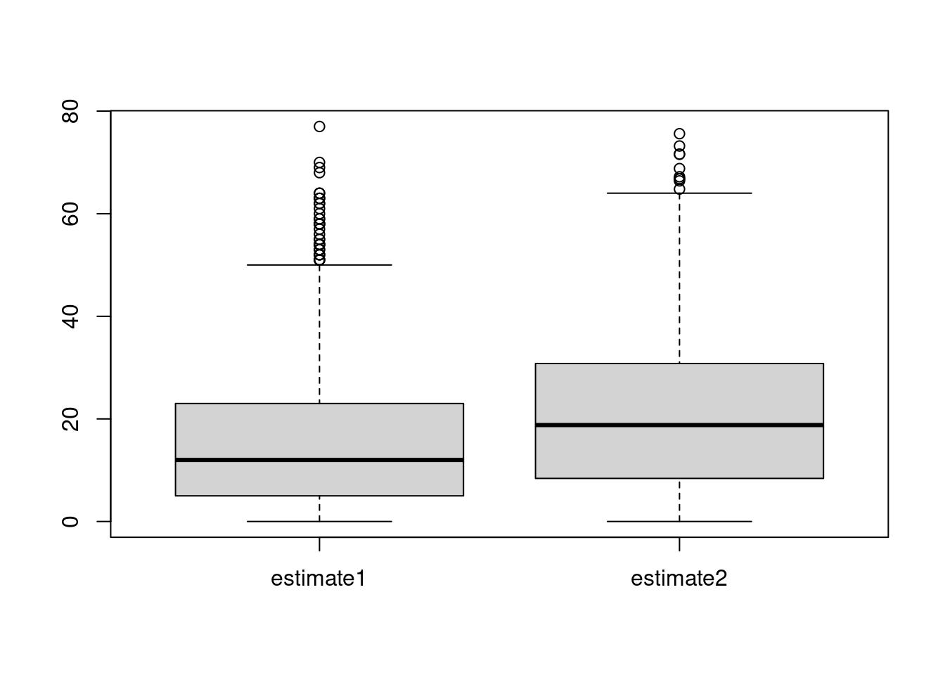
In this case, seems that estimate1 has smaller estimation errors. We can also find the sample mean of the absolute errors and its standard error:
c(mean(absolute.error["estimate1", ]), sd(absolute.error["estimate1", ]) / sqrt(1000))## [1] 15.7170000 0.4511901c(mean(absolute.error["estimate2", ]), sd(absolute.error["estimate2", ]) / sqrt(1000))## [1] 21.463200 0.489799Again, the estimate1 looks better than the estimate2.