2.3 R basics
So let’s get started with R programming!
2.3.1 Introduction to R
R is an Open Source, powerful, flexible and extensible statistical language. It is used by many companies (Google, Microsoft, Facebook, BBVA, etc…) and universities by Statisticians and Data Scientists in software development. Unlike traditional spreadsheets, in R programming sentences are written instead of the classic formulas. It is necessary to know the structure of the data. Prototypes can be made with a few lines of code.
2.3.2 R History
R is an implementation of the statistical language S (combined with the programming language Scheme). S was developed in the AT&T labs by John Chambers in the late 1970s. The two main implementations of S are:
- R
- S+ (S-PLUS)
There are usually several releases a year (usually the most important in April):
- 3.1.0 (Spring Dance) 10/04/2014
- 3.2.0 (Full of Ingredients) 16/04/2015
- 3.5.0 (Joy in Playing) 23/04/2018
- 4.0.0 (Bunny-Wunnies Freak Out) 24/04/2020
- 4.1.0 (Camp Pontanezen) 18/05/2021
2.3.3 R Advantages
R is a great software for solving data analysis problems. There are many packages for data processing, statistical modelling, data mining and graphics. There is a community of users creating packages called the R project.
R is very useful for making graphs, analyzing data and obtaining statistical models with data that fit in the RAM memory of the PC. There are limitations, from a memory point of view, with large volumes of data. It is very common to use another resources to prepare the data:
- Small or medium volumes: Python, Julia, Perl…
- Large Volumes: Spark, Hadoop, Pig, Hive…
2.3.4 What do we mean by R?
By R we usually mean:
- The programming language.
- The interpreter who executes the code written in R.
- The graphics generation system of R.
- The R programming IDE, or also known as RStudio (includes the R interpreter, graphics system, package manager and user interface).
2.3.5 Console Mode
To open the R console, run from the command line (Terminal in Mac):
$>R
The console opens, which allows you to write commands interactively. Each of these commands is called expressions. The R interpreter reads these expressions and responds with the result or an error message. The command interface will store the steps followed when analyzing the data.
The history() command displays the history of commands entered during the R session. Names of variables, packages, directories, etc. are auto-completed using tabulator. If the name of a function is written in the console, its code is displayed. For example: history
history## function (max.show = 25, reverse = FALSE, pattern, ...)
## {
## file1 <- tempfile("Rrawhist")
## savehistory(file1)
## rawhist <- readLines(file1)
## unlink(file1)
## if (!missing(pattern))
## rawhist <- unique(grep(pattern, rawhist, value = TRUE,
## ...))
## nlines <- length(rawhist)
## if (nlines) {
## inds <- max(1, nlines - max.show):nlines
## if (reverse)
## inds <- rev(inds)
## }
## else inds <- integer()
## file2 <- tempfile("hist")
## writeLines(rawhist[inds], file2)
## file.show(file2, title = "R History", delete.file = TRUE)
## }
## <bytecode: 0x55bb067cb8a0>
## <environment: namespace:utils>2.3.6 Getting help in R
The simplest way to get help in R is to click on the Help button on the toolbar of the RGui window (this stands for R’s Graphic User Interface).
However, if you know the name of the function you want help with, you just type a question mark ? at the command line prompt followed by the name of the function. So to get help on read.table, just type:
?read.tableSometimes you cannot remember the precise name of the function, but you know the subject on which you want help (e.g. data input in this case). Use the help.search function (without a question mark) with your query in double quotes like this:
help.search("read tables")Other useful functions are find and apropos. The find function tells you what package something is in:
find("mean")## [1] "package:base"while apropos returns a character vector giving the names of all objects in the search list that match your (potentially partial) enquiry:
apropos("lm")## [1] ".colMeans" ".lm.fit" "colMeans" "confint.lm"
## [5] "contr.helmert" "dummy.coef.lm" "glm" "glm.control"
## [9] "glm.fit" "KalmanForecast" "KalmanLike" "KalmanRun"
## [13] "KalmanSmooth" "kappa.lm" "lm" "lm.fit"
## [17] "lm.influence" "lm.wfit" "model.matrix.lm" "nlm"
## [21] "nlminb" "predict.glm" "predict.lm" "residuals.glm"
## [25] "residuals.lm" "summary.glm" "summary.lm"To see a worked example just type the function name (e.g. linear models, lm) and you will see the printed and graphical output produced by the lm function:
example(lm)##
## lm> require(graphics)
##
## lm> ## Annette Dobson (1990) "An Introduction to Generalized Linear Models".
## lm> ## Page 9: Plant Weight Data.
## lm> ctl <- c(4.17,5.58,5.18,6.11,4.50,4.61,5.17,4.53,5.33,5.14)
##
## lm> trt <- c(4.81,4.17,4.41,3.59,5.87,3.83,6.03,4.89,4.32,4.69)
##
## lm> group <- gl(2, 10, 20, labels = c("Ctl","Trt"))
##
## lm> weight <- c(ctl, trt)
##
## lm> lm.D9 <- lm(weight ~ group)
##
## lm> lm.D90 <- lm(weight ~ group - 1) # omitting intercept
##
## lm> ## No test:
## lm> ##D anova(lm.D9)
## lm> ##D summary(lm.D90)
## lm> ## End(No test)
## lm> opar <- par(mfrow = c(2,2), oma = c(0, 0, 1.1, 0))
##
## lm> plot(lm.D9, las = 1) # Residuals, Fitted, ...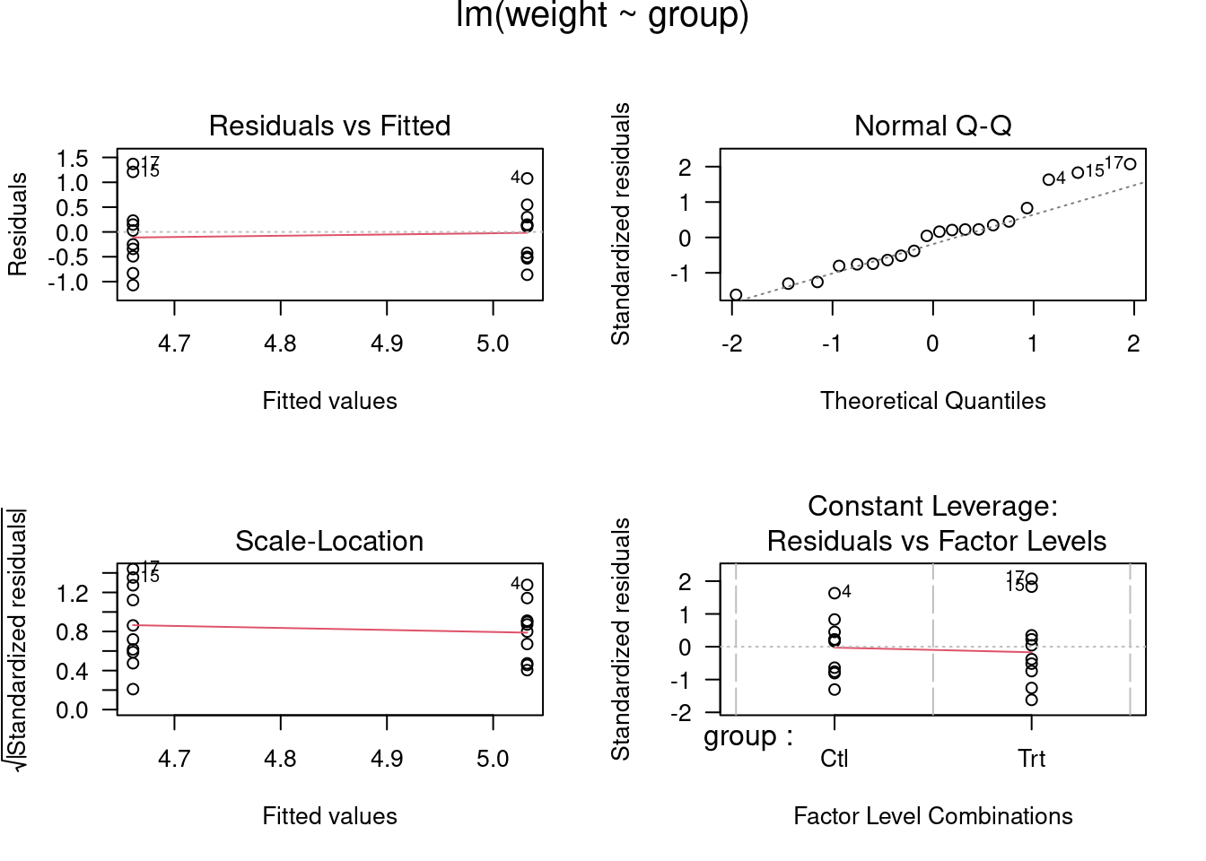
##
## lm> par(opar)
##
## lm> ## Don't show:
## lm> ## model frame :
## lm> stopifnot(identical(lm(weight ~ group, method = "model.frame"),
## lm+                     model.frame(lm.D9)))
##
## lm> ## End(Don't show)
## lm> ### less simple examples in "See Also" above
## lm>
## lm>
## lm>
Demonstrations of R functions can be useful for seeing the range of things that R can do. Here are some for you to try:
#demo(persp)
#demo(graphics)
#demo(Hershey)
#demo(plotmath)
2.3.7 Packages in R
Finding your way around the contributed packages can be tricky, simply because there are so many of them, and the name of the package is not always as indicative of its function as you might hope. There is no comprehensive cross-referenced index, but there is a very helpful feature called ‘Task Views’ on CRAN, which explains the packages available under a limited number of usefully descriptive headings.
2.3.8 Built-in R libraries
To use one of the built-in libraries, simply type the library function with the name of the library in brackets. Thus, to load the dplyr library type:
library(dplyr)##
## Attaching package: 'dplyr'## The following object is masked from 'package:gridExtra':
##
## combine## The following object is masked from 'package:simmer':
##
## select## The following objects are masked from 'package:stats':
##
## filter, lag## The following objects are masked from 'package:base':
##
## intersect, setdiff, setequal, union2.3.9 Contents of Packages
It is easy to use the help function to discover the contents of library packages. Here is how you find out about the contents of the dplyr library:
library(help=dplyr)Then, to find out how to use, say, mutate (mutate), just type:
?mutate2.3.10 Installing Packages
The base package does not contain some of the libraries referred to in this course, but downloading these is very simple. Before you start, you should check whether you need to “Run as administrator” before you can install packages (right click on the R icon to find this).
Run the R program, then from the command line use the install.packages function to download the libraries you want. For example, to install the ggplot2 package type this:
#install.packages("ggplot2")2.3.11 Command line versus scripts
When writing functions and other multi-line sections of input you will find it useful to use a text editor rather than execute everything directly at the command line.
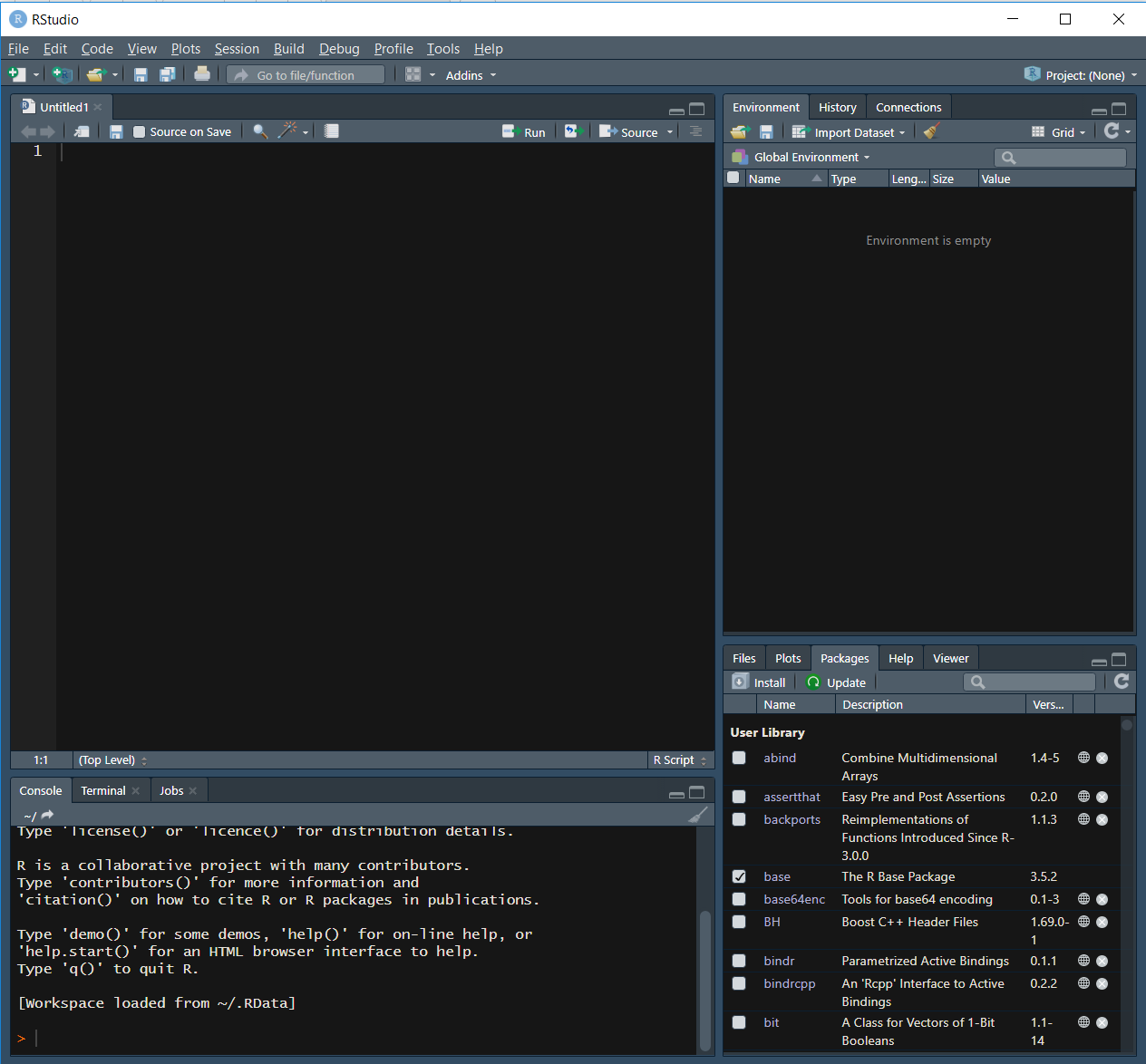
Currently, most users prefer to use an IDE rather than executable text files. The most famous IDE for using R is Rstudio.
2.3.12 RStudio
Programming IDE to develop projects in R: https://www.rstudio.com/
There are two versions:
- RStudio Desktop
- RStudio Server (RStudio Desktop interface in web version)
Both versions have open source (free) and commercial (with support included) versions.
Allows the complete management of a software project:
- Console R
- File management
- Help
- Package management (installation, update, etc.)
- Review of command history
2.3.13 Working Directory
As we have mentioned, R is a programming language that allows us to perform certain actions through an IDE installed in our computer.
In many cases we will need to store data or code sets to use them later. We may also need to read a data set from an external format or even write it. To do all these things, we need to know where we are on the computer, in other words, which folder we are currently in.
We will call this location the working directory. We are going to place there all the resources we need to work with R.
We will use the function setwd() to indicate our location to the R session we are working at.
Example:
setwd("C://User/Desktop/My_Working_Directory")2.3.14 Exercise: Set up your Working Directory
Try to start getting familiar with Rstudio and to set your working directory in a folder that is suitable for the rest of the course.
Remember, within this folder you can create sub-folders for each session in which you can include all the necessary material.